Free Statistics

of Irreproducible Research!

Author's title

Author*Unverified author*
R Software Modulerwasp_smp.wasp
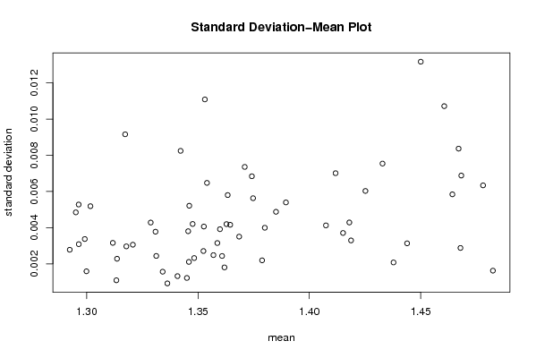
Title produced by softwareStandard Deviation-Mean Plot
Date of computationSun, 11 May 2008 14:55:13 -0600
Cite this page as followsStatistical Computations at FreeStatistics.org, Office for Research Development and Education, URL https://freestatistics.org/blog/index.php?v=date/2008/May/11/t1210539350jkj9th9qdx83ikb.htm/, Retrieved Sun, 19 May 2024 18:48:05 +0000
Statistical Computations at FreeStatistics.org, Office for Research Development and Education, URL https://freestatistics.org/blog/index.php?pk=12289, Retrieved Sun, 19 May 2024 18:48:05 +0000
QR Codes:

Original text written by user:
IsPrivate?No (this computation is public)
User-defined keywords
Estimated Impact209
Family? (F = Feedback message, R = changed R code, M = changed R Module, P = changed Parameters, D = changed Data)
-       [Standard Deviation-Mean Plot] [Referentiewisselk...] [2008-05-11 20:55:13] [ac672cea6030988b680da60b641124d2] [Current]
Feedback Forum

Post a new message
Dataseries X:
1,327
1,3231
1,3106
1,3084
1,3006
1,3018
1,2988
1,2984
1,2893
1,2941
1,2953
1,2909
1,2922
1,2958
1,2936
1,304
1,3005
1,2978
1,2901
1,2921
1,2972
1,2954
1,302
1,302
1,2925
1,2955
1,2987
1,2991
1,3007
1,2956
1,3022
1,3082
1,3137
1,3119
1,3132
1,3145
1,3145
1,3106
1,3134
1,316
1,323
1,3211
1,3225
1,3163
1,3083
1,31
1,3135
1,3152
1,3155
1,3156
1,3218
1,3183
1,3226
1,3325
1,3303
1,3296
1,3293
1,3351
1,3327
1,3265
1,3347
1,3348
1,3352
1,3318
1,3366
1,3358
1,3352
1,3373
1,3426
1,3418
1,3467
1,3532
1,355
1,3549
1,3577
1,3601
1,3606
1,3557
1,3582
1,3649
1,3596
1,3643
1,3605
1,3588
1,3613
1,3561
1,3615
1,3558
1,3535
1,3527
1,3486
1,3549
1,3538
1,3574
1,3516
1,3477
1,3444
1,3454
1,349
1,3448
1,3441
1,3453
1,3509
1,342
1,3453
1,3436
1,3482
1,3532
1,3513
1,347
1,3349
1,3355
1,3345
1,3287
1,3304
1,3314
1,3404
1,3403
1,3427
1,3397
1,3441
1,3461
1,346
1,3438
1,3467
1,3505
1,3588
1,3601
1,3618
1,364
1,3596
1,3621
1,3666
1,3753
1,3788
1,3782
1,3781
1,3771
1,3779
1,382
1,3803
1,3821
1,3833
1,3743
1,3722
1,3651
1,3659
1,3707
1,3663
1,3664
1,3694
1,3818
1,3794
1,3794
1,3729
1,365
1,3651
1,3591
1,3476
1,3405
1,3454
1,3476
1,3508
1,3493
1,3574
1,3615
1,3658
1,3664
1,3631
1,361
1,3705
1,3632
1,358
1,3588
1,3669
1,3696
1,3795
1,3824
1,3885
1,3897
1,386
1,3877
1,3867
1,3975
1,403
1,4049
1,4113
1,4106
1,4127
1,418
1,4179
1,4232
1,4165
1,4195
1,4109
1,4136
1,4089
1,4037
1,4146
1,4199
1,4173
1,4226
1,415
1,42
1,4299
1,4288
1,4166
1,4254
1,423
1,4309
1,4384
1,4391
1,4407
1,4447
1,4423
1,4479
1,4488
1,4547
1,4722
1,4666
1,4683
1,4579
1,4607
1,47
1,4639
1,4651
1,4654
1,4785
1,4814
1,4829
1,4809
1,4845
1,4874
1,4747
1,4738
1,4761
1,4666
1,4741
1,472
1,4554
1,4649
1,4718
1,4672
1,4675
1,4683
1,4509
1,4393
1,4416
1,4385
1,4349
1,438
1,4398
1,4516
1,4692
1,4721


Summary of computational transaction
Raw Inputview raw input (R code)
Raw Outputview raw output of R engine
Computing time3 seconds
R Server'Sir Ronald Aylmer Fisher' @ 193.190.124.24

\begin{tabular}{lllllllll}
\hline
Summary of computational transaction \tabularnewline
Raw Input & view raw input (R code)  \tabularnewline
Raw Output & view raw output of R engine  \tabularnewline
Computing time & 3 seconds \tabularnewline
R Server & 'Sir Ronald Aylmer Fisher' @ 193.190.124.24 \tabularnewline
\hline
\end{tabular}
%Source: https://freestatistics.org/blog/index.php?pk=12289&T=0

[TABLE]
[ROW][C]Summary of computational transaction[/C][/ROW]
[ROW][C]Raw Input[/C][C]view raw input (R code) [/C][/ROW]
[ROW][C]Raw Output[/C][C]view raw output of R engine [/C][/ROW]
[ROW][C]Computing time[/C][C]3 seconds[/C][/ROW]
[ROW][C]R Server[/C][C]'Sir Ronald Aylmer Fisher' @ 193.190.124.24[/C][/ROW]
[/TABLE]
Source: https://freestatistics.org/blog/index.php?pk=12289&T=0

Globally Unique Identifier (entire table): ba.freestatistics.org/blog/index.php?pk=12289&T=0

As an alternative you can also use a QR Code:  

The GUIDs for individual cells are displayed in the table below:

Summary of computational transaction
Raw Inputview raw input (R code)
Raw Outputview raw output of R engine
Computing time3 seconds
R Server'Sir Ronald Aylmer Fisher' @ 193.190.124.24


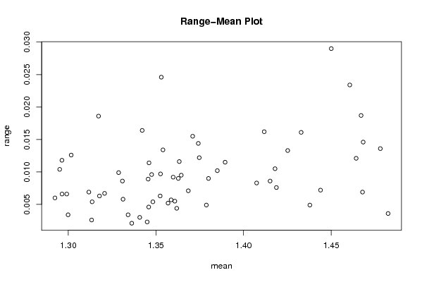
Standard Deviation-Mean Plot
SectionMeanStandard DeviationRange
11.3172750.009162013970738070.0185999999999999
21.29990.001587450786638790.00340000000000007
31.29240.002778488797889980.006
41.29640.005278888771954440.0118000000000000
51.2951250.004845874534075340.0104000000000000
61.299150.003371943060017480.00659999999999994
71.296450.003087069808086590.00659999999999994
81.3016750.005186761995696330.0125999999999999
91.3133250.001090489186863690.00259999999999994
101.3136250.002280898945591440.00540000000000007
111.3207250.003057640702676900.00669999999999993
121.311750.003158586181611360.0068999999999999
131.31780.002965355515504610.0063000000000002
141.328750.004282133424668910.00990000000000002
151.33090.00377712412645740.00859999999999994
161.3341250.001564981363041260.00339999999999985
171.3362250.0009178779875342730.00209999999999999
181.3460750.005212405075074860.0113999999999999
191.3569250.002482438317461320.00520000000000009
201.359850.003916205646626190.0092000000000001
211.36080.002434474618201400.00550000000000006
221.3586750.003149999999999980.00570000000000004
231.3524250.002707243370416950.00629999999999997
241.3526250.004061506288722630.00970000000000004
251.34590.002107130750570530.00459999999999994
261.3455750.003802959373961250.0088999999999999
271.3475750.004203470788130550.00960000000000005
281.3421750.00824676704331260.0164000000000000
291.331250.002436527583809940.00580000000000003
301.3407750.001320037878244430.00300000000000011
311.3450.001219289410544790.00229999999999997
321.3540250.006475273481998030.0134000000000001
331.3618750.001802544497832700.00440000000000018
341.3747250.005628128759484220.0122
351.3787750.002192981228069780.0048999999999999
361.380.003994996871087610.0089999999999999
371.3684750.003504639781775080.0071000000000001
381.3709750.007358611735012640.0154999999999998
391.3741750.006841235268575390.0144000000000000
401.3530750.01109064921454100.0246000000000000
411.3482750.002320021551624070.00540000000000007
421.3627750.004195533339159660.00900000000000012
431.364450.004158926143449410.00950000000000006
441.3633250.005801939330947830.0115999999999998
451.3850250.004876730462102660.0102000000000000
461.3894750.005395291156802080.0115000000000001
471.407450.004125126260693930.00829999999999997
481.417950.004286801449410330.0105000000000000
491.4151250.003706188518320850.00859999999999994
501.4117750.007011122116561180.0162
511.4187250.003293807320816860.00760000000000005
521.4251750.0060290270082880.0132999999999999
531.432850.007542987913729290.0161
541.44390.003132624033192170.00719999999999987
551.4605750.01071770342315300.0233999999999999
561.4642250.005842017345632090.0121
571.4682250.006880588637609380.0145999999999999
581.4824250.001623524971576700.00359999999999983
591.4780.006337717780610560.0136000000000001
601.4670250.008369139740737970.0186999999999999
611.467850.002878078062411290.0068999999999999
621.4500250.01317507115730310.0289999999999999
631.43780.002076856599125970.0048999999999999

\begin{tabular}{lllllllll}
\hline
Standard Deviation-Mean Plot \tabularnewline
Section & Mean & Standard Deviation & Range \tabularnewline
1 & 1.317275 & 0.00916201397073807 & 0.0185999999999999 \tabularnewline
2 & 1.2999 & 0.00158745078663879 & 0.00340000000000007 \tabularnewline
3 & 1.2924 & 0.00277848879788998 & 0.006 \tabularnewline
4 & 1.2964 & 0.00527888877195444 & 0.0118000000000000 \tabularnewline
5 & 1.295125 & 0.00484587453407534 & 0.0104000000000000 \tabularnewline
6 & 1.29915 & 0.00337194306001748 & 0.00659999999999994 \tabularnewline
7 & 1.29645 & 0.00308706980808659 & 0.00659999999999994 \tabularnewline
8 & 1.301675 & 0.00518676199569633 & 0.0125999999999999 \tabularnewline
9 & 1.313325 & 0.00109048918686369 & 0.00259999999999994 \tabularnewline
10 & 1.313625 & 0.00228089894559144 & 0.00540000000000007 \tabularnewline
11 & 1.320725 & 0.00305764070267690 & 0.00669999999999993 \tabularnewline
12 & 1.31175 & 0.00315858618161136 & 0.0068999999999999 \tabularnewline
13 & 1.3178 & 0.00296535551550461 & 0.0063000000000002 \tabularnewline
14 & 1.32875 & 0.00428213342466891 & 0.00990000000000002 \tabularnewline
15 & 1.3309 & 0.0037771241264574 & 0.00859999999999994 \tabularnewline
16 & 1.334125 & 0.00156498136304126 & 0.00339999999999985 \tabularnewline
17 & 1.336225 & 0.000917877987534273 & 0.00209999999999999 \tabularnewline
18 & 1.346075 & 0.00521240507507486 & 0.0113999999999999 \tabularnewline
19 & 1.356925 & 0.00248243831746132 & 0.00520000000000009 \tabularnewline
20 & 1.35985 & 0.00391620564662619 & 0.0092000000000001 \tabularnewline
21 & 1.3608 & 0.00243447461820140 & 0.00550000000000006 \tabularnewline
22 & 1.358675 & 0.00314999999999998 & 0.00570000000000004 \tabularnewline
23 & 1.352425 & 0.00270724337041695 & 0.00629999999999997 \tabularnewline
24 & 1.352625 & 0.00406150628872263 & 0.00970000000000004 \tabularnewline
25 & 1.3459 & 0.00210713075057053 & 0.00459999999999994 \tabularnewline
26 & 1.345575 & 0.00380295937396125 & 0.0088999999999999 \tabularnewline
27 & 1.347575 & 0.00420347078813055 & 0.00960000000000005 \tabularnewline
28 & 1.342175 & 0.0082467670433126 & 0.0164000000000000 \tabularnewline
29 & 1.33125 & 0.00243652758380994 & 0.00580000000000003 \tabularnewline
30 & 1.340775 & 0.00132003787824443 & 0.00300000000000011 \tabularnewline
31 & 1.345 & 0.00121928941054479 & 0.00229999999999997 \tabularnewline
32 & 1.354025 & 0.00647527348199803 & 0.0134000000000001 \tabularnewline
33 & 1.361875 & 0.00180254449783270 & 0.00440000000000018 \tabularnewline
34 & 1.374725 & 0.00562812875948422 & 0.0122 \tabularnewline
35 & 1.378775 & 0.00219298122806978 & 0.0048999999999999 \tabularnewline
36 & 1.38 & 0.00399499687108761 & 0.0089999999999999 \tabularnewline
37 & 1.368475 & 0.00350463978177508 & 0.0071000000000001 \tabularnewline
38 & 1.370975 & 0.00735861173501264 & 0.0154999999999998 \tabularnewline
39 & 1.374175 & 0.00684123526857539 & 0.0144000000000000 \tabularnewline
40 & 1.353075 & 0.0110906492145410 & 0.0246000000000000 \tabularnewline
41 & 1.348275 & 0.00232002155162407 & 0.00540000000000007 \tabularnewline
42 & 1.362775 & 0.00419553333915966 & 0.00900000000000012 \tabularnewline
43 & 1.36445 & 0.00415892614344941 & 0.00950000000000006 \tabularnewline
44 & 1.363325 & 0.00580193933094783 & 0.0115999999999998 \tabularnewline
45 & 1.385025 & 0.00487673046210266 & 0.0102000000000000 \tabularnewline
46 & 1.389475 & 0.00539529115680208 & 0.0115000000000001 \tabularnewline
47 & 1.40745 & 0.00412512626069393 & 0.00829999999999997 \tabularnewline
48 & 1.41795 & 0.00428680144941033 & 0.0105000000000000 \tabularnewline
49 & 1.415125 & 0.00370618851832085 & 0.00859999999999994 \tabularnewline
50 & 1.411775 & 0.00701112211656118 & 0.0162 \tabularnewline
51 & 1.418725 & 0.00329380732081686 & 0.00760000000000005 \tabularnewline
52 & 1.425175 & 0.006029027008288 & 0.0132999999999999 \tabularnewline
53 & 1.43285 & 0.00754298791372929 & 0.0161 \tabularnewline
54 & 1.4439 & 0.00313262403319217 & 0.00719999999999987 \tabularnewline
55 & 1.460575 & 0.0107177034231530 & 0.0233999999999999 \tabularnewline
56 & 1.464225 & 0.00584201734563209 & 0.0121 \tabularnewline
57 & 1.468225 & 0.00688058863760938 & 0.0145999999999999 \tabularnewline
58 & 1.482425 & 0.00162352497157670 & 0.00359999999999983 \tabularnewline
59 & 1.478 & 0.00633771778061056 & 0.0136000000000001 \tabularnewline
60 & 1.467025 & 0.00836913974073797 & 0.0186999999999999 \tabularnewline
61 & 1.46785 & 0.00287807806241129 & 0.0068999999999999 \tabularnewline
62 & 1.450025 & 0.0131750711573031 & 0.0289999999999999 \tabularnewline
63 & 1.4378 & 0.00207685659912597 & 0.0048999999999999 \tabularnewline
\hline
\end{tabular}
%Source: https://freestatistics.org/blog/index.php?pk=12289&T=1

[TABLE]
[ROW][C]Standard Deviation-Mean Plot[/C][/ROW]
[ROW][C]Section[/C][C]Mean[/C][C]Standard Deviation[/C][C]Range[/C][/ROW]
[ROW][C]1[/C][C]1.317275[/C][C]0.00916201397073807[/C][C]0.0185999999999999[/C][/ROW]
[ROW][C]2[/C][C]1.2999[/C][C]0.00158745078663879[/C][C]0.00340000000000007[/C][/ROW]
[ROW][C]3[/C][C]1.2924[/C][C]0.00277848879788998[/C][C]0.006[/C][/ROW]
[ROW][C]4[/C][C]1.2964[/C][C]0.00527888877195444[/C][C]0.0118000000000000[/C][/ROW]
[ROW][C]5[/C][C]1.295125[/C][C]0.00484587453407534[/C][C]0.0104000000000000[/C][/ROW]
[ROW][C]6[/C][C]1.29915[/C][C]0.00337194306001748[/C][C]0.00659999999999994[/C][/ROW]
[ROW][C]7[/C][C]1.29645[/C][C]0.00308706980808659[/C][C]0.00659999999999994[/C][/ROW]
[ROW][C]8[/C][C]1.301675[/C][C]0.00518676199569633[/C][C]0.0125999999999999[/C][/ROW]
[ROW][C]9[/C][C]1.313325[/C][C]0.00109048918686369[/C][C]0.00259999999999994[/C][/ROW]
[ROW][C]10[/C][C]1.313625[/C][C]0.00228089894559144[/C][C]0.00540000000000007[/C][/ROW]
[ROW][C]11[/C][C]1.320725[/C][C]0.00305764070267690[/C][C]0.00669999999999993[/C][/ROW]
[ROW][C]12[/C][C]1.31175[/C][C]0.00315858618161136[/C][C]0.0068999999999999[/C][/ROW]
[ROW][C]13[/C][C]1.3178[/C][C]0.00296535551550461[/C][C]0.0063000000000002[/C][/ROW]
[ROW][C]14[/C][C]1.32875[/C][C]0.00428213342466891[/C][C]0.00990000000000002[/C][/ROW]
[ROW][C]15[/C][C]1.3309[/C][C]0.0037771241264574[/C][C]0.00859999999999994[/C][/ROW]
[ROW][C]16[/C][C]1.334125[/C][C]0.00156498136304126[/C][C]0.00339999999999985[/C][/ROW]
[ROW][C]17[/C][C]1.336225[/C][C]0.000917877987534273[/C][C]0.00209999999999999[/C][/ROW]
[ROW][C]18[/C][C]1.346075[/C][C]0.00521240507507486[/C][C]0.0113999999999999[/C][/ROW]
[ROW][C]19[/C][C]1.356925[/C][C]0.00248243831746132[/C][C]0.00520000000000009[/C][/ROW]
[ROW][C]20[/C][C]1.35985[/C][C]0.00391620564662619[/C][C]0.0092000000000001[/C][/ROW]
[ROW][C]21[/C][C]1.3608[/C][C]0.00243447461820140[/C][C]0.00550000000000006[/C][/ROW]
[ROW][C]22[/C][C]1.358675[/C][C]0.00314999999999998[/C][C]0.00570000000000004[/C][/ROW]
[ROW][C]23[/C][C]1.352425[/C][C]0.00270724337041695[/C][C]0.00629999999999997[/C][/ROW]
[ROW][C]24[/C][C]1.352625[/C][C]0.00406150628872263[/C][C]0.00970000000000004[/C][/ROW]
[ROW][C]25[/C][C]1.3459[/C][C]0.00210713075057053[/C][C]0.00459999999999994[/C][/ROW]
[ROW][C]26[/C][C]1.345575[/C][C]0.00380295937396125[/C][C]0.0088999999999999[/C][/ROW]
[ROW][C]27[/C][C]1.347575[/C][C]0.00420347078813055[/C][C]0.00960000000000005[/C][/ROW]
[ROW][C]28[/C][C]1.342175[/C][C]0.0082467670433126[/C][C]0.0164000000000000[/C][/ROW]
[ROW][C]29[/C][C]1.33125[/C][C]0.00243652758380994[/C][C]0.00580000000000003[/C][/ROW]
[ROW][C]30[/C][C]1.340775[/C][C]0.00132003787824443[/C][C]0.00300000000000011[/C][/ROW]
[ROW][C]31[/C][C]1.345[/C][C]0.00121928941054479[/C][C]0.00229999999999997[/C][/ROW]
[ROW][C]32[/C][C]1.354025[/C][C]0.00647527348199803[/C][C]0.0134000000000001[/C][/ROW]
[ROW][C]33[/C][C]1.361875[/C][C]0.00180254449783270[/C][C]0.00440000000000018[/C][/ROW]
[ROW][C]34[/C][C]1.374725[/C][C]0.00562812875948422[/C][C]0.0122[/C][/ROW]
[ROW][C]35[/C][C]1.378775[/C][C]0.00219298122806978[/C][C]0.0048999999999999[/C][/ROW]
[ROW][C]36[/C][C]1.38[/C][C]0.00399499687108761[/C][C]0.0089999999999999[/C][/ROW]
[ROW][C]37[/C][C]1.368475[/C][C]0.00350463978177508[/C][C]0.0071000000000001[/C][/ROW]
[ROW][C]38[/C][C]1.370975[/C][C]0.00735861173501264[/C][C]0.0154999999999998[/C][/ROW]
[ROW][C]39[/C][C]1.374175[/C][C]0.00684123526857539[/C][C]0.0144000000000000[/C][/ROW]
[ROW][C]40[/C][C]1.353075[/C][C]0.0110906492145410[/C][C]0.0246000000000000[/C][/ROW]
[ROW][C]41[/C][C]1.348275[/C][C]0.00232002155162407[/C][C]0.00540000000000007[/C][/ROW]
[ROW][C]42[/C][C]1.362775[/C][C]0.00419553333915966[/C][C]0.00900000000000012[/C][/ROW]
[ROW][C]43[/C][C]1.36445[/C][C]0.00415892614344941[/C][C]0.00950000000000006[/C][/ROW]
[ROW][C]44[/C][C]1.363325[/C][C]0.00580193933094783[/C][C]0.0115999999999998[/C][/ROW]
[ROW][C]45[/C][C]1.385025[/C][C]0.00487673046210266[/C][C]0.0102000000000000[/C][/ROW]
[ROW][C]46[/C][C]1.389475[/C][C]0.00539529115680208[/C][C]0.0115000000000001[/C][/ROW]
[ROW][C]47[/C][C]1.40745[/C][C]0.00412512626069393[/C][C]0.00829999999999997[/C][/ROW]
[ROW][C]48[/C][C]1.41795[/C][C]0.00428680144941033[/C][C]0.0105000000000000[/C][/ROW]
[ROW][C]49[/C][C]1.415125[/C][C]0.00370618851832085[/C][C]0.00859999999999994[/C][/ROW]
[ROW][C]50[/C][C]1.411775[/C][C]0.00701112211656118[/C][C]0.0162[/C][/ROW]
[ROW][C]51[/C][C]1.418725[/C][C]0.00329380732081686[/C][C]0.00760000000000005[/C][/ROW]
[ROW][C]52[/C][C]1.425175[/C][C]0.006029027008288[/C][C]0.0132999999999999[/C][/ROW]
[ROW][C]53[/C][C]1.43285[/C][C]0.00754298791372929[/C][C]0.0161[/C][/ROW]
[ROW][C]54[/C][C]1.4439[/C][C]0.00313262403319217[/C][C]0.00719999999999987[/C][/ROW]
[ROW][C]55[/C][C]1.460575[/C][C]0.0107177034231530[/C][C]0.0233999999999999[/C][/ROW]
[ROW][C]56[/C][C]1.464225[/C][C]0.00584201734563209[/C][C]0.0121[/C][/ROW]
[ROW][C]57[/C][C]1.468225[/C][C]0.00688058863760938[/C][C]0.0145999999999999[/C][/ROW]
[ROW][C]58[/C][C]1.482425[/C][C]0.00162352497157670[/C][C]0.00359999999999983[/C][/ROW]
[ROW][C]59[/C][C]1.478[/C][C]0.00633771778061056[/C][C]0.0136000000000001[/C][/ROW]
[ROW][C]60[/C][C]1.467025[/C][C]0.00836913974073797[/C][C]0.0186999999999999[/C][/ROW]
[ROW][C]61[/C][C]1.46785[/C][C]0.00287807806241129[/C][C]0.0068999999999999[/C][/ROW]
[ROW][C]62[/C][C]1.450025[/C][C]0.0131750711573031[/C][C]0.0289999999999999[/C][/ROW]
[ROW][C]63[/C][C]1.4378[/C][C]0.00207685659912597[/C][C]0.0048999999999999[/C][/ROW]
[/TABLE]
Source: https://freestatistics.org/blog/index.php?pk=12289&T=1

Globally Unique Identifier (entire table): ba.freestatistics.org/blog/index.php?pk=12289&T=1

As an alternative you can also use a QR Code:  

The GUIDs for individual cells are displayed in the table below:

Standard Deviation-Mean Plot
SectionMeanStandard DeviationRange
11.3172750.009162013970738070.0185999999999999
21.29990.001587450786638790.00340000000000007
31.29240.002778488797889980.006
41.29640.005278888771954440.0118000000000000
51.2951250.004845874534075340.0104000000000000
61.299150.003371943060017480.00659999999999994
71.296450.003087069808086590.00659999999999994
81.3016750.005186761995696330.0125999999999999
91.3133250.001090489186863690.00259999999999994
101.3136250.002280898945591440.00540000000000007
111.3207250.003057640702676900.00669999999999993
121.311750.003158586181611360.0068999999999999
131.31780.002965355515504610.0063000000000002
141.328750.004282133424668910.00990000000000002
151.33090.00377712412645740.00859999999999994
161.3341250.001564981363041260.00339999999999985
171.3362250.0009178779875342730.00209999999999999
181.3460750.005212405075074860.0113999999999999
191.3569250.002482438317461320.00520000000000009
201.359850.003916205646626190.0092000000000001
211.36080.002434474618201400.00550000000000006
221.3586750.003149999999999980.00570000000000004
231.3524250.002707243370416950.00629999999999997
241.3526250.004061506288722630.00970000000000004
251.34590.002107130750570530.00459999999999994
261.3455750.003802959373961250.0088999999999999
271.3475750.004203470788130550.00960000000000005
281.3421750.00824676704331260.0164000000000000
291.331250.002436527583809940.00580000000000003
301.3407750.001320037878244430.00300000000000011
311.3450.001219289410544790.00229999999999997
321.3540250.006475273481998030.0134000000000001
331.3618750.001802544497832700.00440000000000018
341.3747250.005628128759484220.0122
351.3787750.002192981228069780.0048999999999999
361.380.003994996871087610.0089999999999999
371.3684750.003504639781775080.0071000000000001
381.3709750.007358611735012640.0154999999999998
391.3741750.006841235268575390.0144000000000000
401.3530750.01109064921454100.0246000000000000
411.3482750.002320021551624070.00540000000000007
421.3627750.004195533339159660.00900000000000012
431.364450.004158926143449410.00950000000000006
441.3633250.005801939330947830.0115999999999998
451.3850250.004876730462102660.0102000000000000
461.3894750.005395291156802080.0115000000000001
471.407450.004125126260693930.00829999999999997
481.417950.004286801449410330.0105000000000000
491.4151250.003706188518320850.00859999999999994
501.4117750.007011122116561180.0162
511.4187250.003293807320816860.00760000000000005
521.4251750.0060290270082880.0132999999999999
531.432850.007542987913729290.0161
541.44390.003132624033192170.00719999999999987
551.4605750.01071770342315300.0233999999999999
561.4642250.005842017345632090.0121
571.4682250.006880588637609380.0145999999999999
581.4824250.001623524971576700.00359999999999983
591.4780.006337717780610560.0136000000000001
601.4670250.008369139740737970.0186999999999999
611.467850.002878078062411290.0068999999999999
621.4500250.01317507115730310.0289999999999999
631.43780.002076856599125970.0048999999999999


Regression: S.E.(k) = alpha + beta * Mean(k)
alpha-0.0187013094929634
beta0.0168835822350529
S.D.0.00580115427991047
T-STAT2.91038324795482
p-value0.00503300846337504

\begin{tabular}{lllllllll}
\hline
Regression: S.E.(k) = alpha + beta * Mean(k) \tabularnewline
alpha & -0.0187013094929634 \tabularnewline
beta & 0.0168835822350529 \tabularnewline
S.D. & 0.00580115427991047 \tabularnewline
T-STAT & 2.91038324795482 \tabularnewline
p-value & 0.00503300846337504 \tabularnewline
\hline
\end{tabular}
%Source: https://freestatistics.org/blog/index.php?pk=12289&T=2

[TABLE]
[ROW][C]Regression: S.E.(k) = alpha + beta * Mean(k)[/C][/ROW]
[ROW][C]alpha[/C][C]-0.0187013094929634[/C][/ROW]
[ROW][C]beta[/C][C]0.0168835822350529[/C][/ROW]
[ROW][C]S.D.[/C][C]0.00580115427991047[/C][/ROW]
[ROW][C]T-STAT[/C][C]2.91038324795482[/C][/ROW]
[ROW][C]p-value[/C][C]0.00503300846337504[/C][/ROW]
[/TABLE]
Source: https://freestatistics.org/blog/index.php?pk=12289&T=2

Globally Unique Identifier (entire table): ba.freestatistics.org/blog/index.php?pk=12289&T=2

As an alternative you can also use a QR Code:  

The GUIDs for individual cells are displayed in the table below:

Regression: S.E.(k) = alpha + beta * Mean(k)
alpha-0.0187013094929634
beta0.0168835822350529
S.D.0.00580115427991047
T-STAT2.91038324795482
p-value0.00503300846337504


Regression: ln S.E.(k) = alpha + beta * ln Mean(k)
alpha-7.14391792948849
beta4.98046988493984
S.D.1.85188030910744
T-STAT2.6894124098875
p-value0.00921851489043492
Lambda-3.98046988493984

\begin{tabular}{lllllllll}
\hline
Regression: ln S.E.(k) = alpha + beta * ln Mean(k) \tabularnewline
alpha & -7.14391792948849 \tabularnewline
beta & 4.98046988493984 \tabularnewline
S.D. & 1.85188030910744 \tabularnewline
T-STAT & 2.6894124098875 \tabularnewline
p-value & 0.00921851489043492 \tabularnewline
Lambda & -3.98046988493984 \tabularnewline
\hline
\end{tabular}
%Source: https://freestatistics.org/blog/index.php?pk=12289&T=3

[TABLE]
[ROW][C]Regression: ln S.E.(k) = alpha + beta * ln Mean(k)[/C][/ROW]
[ROW][C]alpha[/C][C]-7.14391792948849[/C][/ROW]
[ROW][C]beta[/C][C]4.98046988493984[/C][/ROW]
[ROW][C]S.D.[/C][C]1.85188030910744[/C][/ROW]
[ROW][C]T-STAT[/C][C]2.6894124098875[/C][/ROW]
[ROW][C]p-value[/C][C]0.00921851489043492[/C][/ROW]
[ROW][C]Lambda[/C][C]-3.98046988493984[/C][/ROW]
[/TABLE]
Source: https://freestatistics.org/blog/index.php?pk=12289&T=3

Globally Unique Identifier (entire table): ba.freestatistics.org/blog/index.php?pk=12289&T=3

As an alternative you can also use a QR Code:  

The GUIDs for individual cells are displayed in the table below:

Regression: ln S.E.(k) = alpha + beta * ln Mean(k)
alpha-7.14391792948849
beta4.98046988493984
S.D.1.85188030910744
T-STAT2.6894124098875
p-value0.00921851489043492
Lambda-3.98046988493984


Parameters (Session):
par1 = 4 ;
Parameters (R input):
par1 = 4 ;
R code (references can be found in the software module):
par1 <- as.numeric(par1)
(n <- length(x))
(np <- floor(n / par1))
arr <- array(NA,dim=c(par1,np))
j <- 0
k <- 1
for (i in 1:(np*par1))
{
j = j + 1
arr[j,k] <- x[i]
if (j == par1) {
j = 0
k=k+1
}
}
arr
arr.mean <- array(NA,dim=np)
arr.sd <- array(NA,dim=np)
arr.range <- array(NA,dim=np)
for (j in 1:np)
{
arr.mean[j] <- mean(arr[,j],na.rm=TRUE)
arr.sd[j] <- sd(arr[,j],na.rm=TRUE)
arr.range[j] <- max(arr[,j],na.rm=TRUE) - min(arr[,j],na.rm=TRUE)
}
arr.mean
arr.sd
arr.range
(lm1 <- lm(arr.sd~arr.mean))
(lnlm1 <- lm(log(arr.sd)~log(arr.mean)))
(lm2 <- lm(arr.range~arr.mean))
bitmap(file='test1.png')
plot(arr.mean,arr.sd,main='Standard Deviation-Mean Plot',xlab='mean',ylab='standard deviation')
dev.off()
bitmap(file='test2.png')
plot(arr.mean,arr.range,main='Range-Mean Plot',xlab='mean',ylab='range')
dev.off()
load(file='createtable')
a<-table.start()
a<-table.row.start(a)
a<-table.element(a,'Standard Deviation-Mean Plot',4,TRUE)
a<-table.row.end(a)
a<-table.row.start(a)
a<-table.element(a,'Section',header=TRUE)
a<-table.element(a,'Mean',header=TRUE)
a<-table.element(a,'Standard Deviation',header=TRUE)
a<-table.element(a,'Range',header=TRUE)
a<-table.row.end(a)
for (j in 1:np) {
a<-table.row.start(a)
a<-table.element(a,j,header=TRUE)
a<-table.element(a,arr.mean[j])
a<-table.element(a,arr.sd[j] )
a<-table.element(a,arr.range[j] )
a<-table.row.end(a)
}
a<-table.end(a)
table.save(a,file='mytable.tab')
a<-table.start()
a<-table.row.start(a)
a<-table.element(a,'Regression: S.E.(k) = alpha + beta * Mean(k)',2,TRUE)
a<-table.row.end(a)
a<-table.row.start(a)
a<-table.element(a,'alpha',header=TRUE)
a<-table.element(a,lm1$coefficients[[1]])
a<-table.row.end(a)
a<-table.row.start(a)
a<-table.element(a,'beta',header=TRUE)
a<-table.element(a,lm1$coefficients[[2]])
a<-table.row.end(a)
a<-table.row.start(a)
a<-table.element(a,'S.D.',header=TRUE)
a<-table.element(a,summary(lm1)$coefficients[2,2])
a<-table.row.end(a)
a<-table.row.start(a)
a<-table.element(a,'T-STAT',header=TRUE)
a<-table.element(a,summary(lm1)$coefficients[2,3])
a<-table.row.end(a)
a<-table.row.start(a)
a<-table.element(a,'p-value',header=TRUE)
a<-table.element(a,summary(lm1)$coefficients[2,4])
a<-table.row.end(a)
a<-table.end(a)
table.save(a,file='mytable1.tab')
a<-table.start()
a<-table.row.start(a)
a<-table.element(a,'Regression: ln S.E.(k) = alpha + beta * ln Mean(k)',2,TRUE)
a<-table.row.end(a)
a<-table.row.start(a)
a<-table.element(a,'alpha',header=TRUE)
a<-table.element(a,lnlm1$coefficients[[1]])
a<-table.row.end(a)
a<-table.row.start(a)
a<-table.element(a,'beta',header=TRUE)
a<-table.element(a,lnlm1$coefficients[[2]])
a<-table.row.end(a)
a<-table.row.start(a)
a<-table.element(a,'S.D.',header=TRUE)
a<-table.element(a,summary(lnlm1)$coefficients[2,2])
a<-table.row.end(a)
a<-table.row.start(a)
a<-table.element(a,'T-STAT',header=TRUE)
a<-table.element(a,summary(lnlm1)$coefficients[2,3])
a<-table.row.end(a)
a<-table.row.start(a)
a<-table.element(a,'p-value',header=TRUE)
a<-table.element(a,summary(lnlm1)$coefficients[2,4])
a<-table.row.end(a)
a<-table.row.start(a)
a<-table.element(a,'Lambda',header=TRUE)
a<-table.element(a,1-lnlm1$coefficients[[2]])
a<-table.row.end(a)
a<-table.end(a)
table.save(a,file='mytable2.tab')