Repository of Reproducible Computations

Free Statistics

of Irreproducible Research!

Author's title

Author

*Unverified author*

R Software Module

rwasp_autocorrelation.wasp

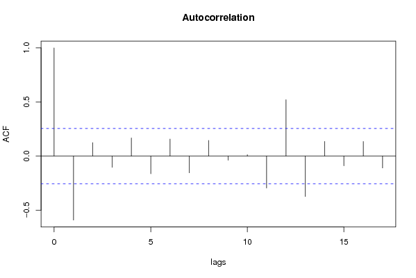
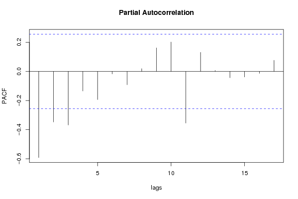
Title produced by software

(Partial) Autocorrelation Function

Date of computation

Wed, 24 Dec 2008 07:06:47 -0700

Cite this page as follows

Statistical Computations at FreeStatistics.org, Office for Research Development and Education, URL https://freestatistics.org/blog/index.php?v=date/2008/Dec/24/t1230127629jlrg3wp5lf4ndyl.htm/, Retrieved Sun, 19 May 2024 11:38:35 +0000

Statistical Computations at FreeStatistics.org, Office for Research Development and Education, URL https://freestatistics.org/blog/index.php?pk=36574, Retrieved Sun, 19 May 2024 11:38:35 +0000

QR Codes:

Paste this QR Code to cite your computation.

Original text written by user:

IsPrivate?

No (this computation is public)

User-defined keywords

Estimated Impact

193

Family? (F = Feedback message, R = changed R code, M = changed R Module, P = changed Parameters, D = changed Data)

-     [(Partial) Autocorrelation Function] [autocorrelatie: e...] [2007-12-15 09:28:58] [707a919fab5d6f3020ea3c395672cd86]
- R PD    [(Partial) Autocorrelation Function] [Nick Mulkens] [2008-12-24 14:06:47] [d41d8cd98f00b204e9800998ecf8427e] [Current]

Feedback Forum

Post a new message

Dataseries X:

Download CSV

Histogram

Boxplots

Summary of computational transaction
Raw Input	view raw input (R code)
Raw Output	view raw output of R engine
Computing time	2 seconds
R Server	'Sir Ronald Aylmer Fisher' @ 193.190.124.24

\begin{tabular}{lllllllll}
\hline
Summary of computational transaction \tabularnewline
Raw Input & view raw input (R code)  \tabularnewline
Raw Output & view raw output of R engine  \tabularnewline
Computing time & 2 seconds \tabularnewline
R Server & 'Sir Ronald Aylmer Fisher' @ 193.190.124.24 \tabularnewline
\hline
\end{tabular}
%Source: https://freestatistics.org/blog/index.php?pk=36574&T=0

[TABLE]
[ROW][C]Summary of computational transaction[/C][/ROW]
[ROW][C]Raw Input[/C][C]view raw input (R code) [/C][/ROW]
[ROW][C]Raw Output[/C][C]view raw output of R engine [/C][/ROW]
[ROW][C]Computing time[/C][C]2 seconds[/C][/ROW]
[ROW][C]R Server[/C][C]'Sir Ronald Aylmer Fisher' @ 193.190.124.24[/C][/ROW]
[/TABLE]
Source: https://freestatistics.org/blog/index.php?pk=36574&T=0

Globally Unique Identifier (entire table): ba.freestatistics.org/blog/index.php?pk=36574&T=0

As an alternative you can also use a QR Code:

The GUIDs for individual cells are displayed in the table below:

Summary of computational transaction
Raw Input	view raw input (R code)
Raw Output	view raw output of R engine
Computing time	2 seconds
R Server	'Sir Ronald Aylmer Fisher' @ 193.190.124.24

Autocorrelation Function
Time lag k	ACF(k)	T-STAT	P-value
1	-0.591359	-4.5423	1.4e-05
2	0.1241	0.9532	0.172182
3	-0.10434	-0.8015	0.213043
4	0.168408	1.2936	0.100429
5	-0.163729	-1.2576	0.106742
6	0.157554	1.2102	0.115514
7	-0.154471	-1.1865	0.120087
8	0.144791	1.1122	0.13529
9	-0.038193	-0.2934	0.385135
10	0.013026	0.1001	0.46032
11	-0.294702	-2.2636	0.013644
12	0.521105	4.0027	8.9e-05
13	-0.373482	-2.8688	0.002855
14	0.135337	1.0395	0.151396
15	-0.089422	-0.6869	0.247429
16	0.134927	1.0364	0.152123
17	-0.109609	-0.8419	0.201615

\begin{tabular}{lllllllll}
\hline
Autocorrelation Function \tabularnewline
Time lag k & ACF(k) & T-STAT & P-value \tabularnewline
1 & -0.591359 & -4.5423 & 1.4e-05 \tabularnewline
2 & 0.1241 & 0.9532 & 0.172182 \tabularnewline
3 & -0.10434 & -0.8015 & 0.213043 \tabularnewline
4 & 0.168408 & 1.2936 & 0.100429 \tabularnewline
5 & -0.163729 & -1.2576 & 0.106742 \tabularnewline
6 & 0.157554 & 1.2102 & 0.115514 \tabularnewline
7 & -0.154471 & -1.1865 & 0.120087 \tabularnewline
8 & 0.144791 & 1.1122 & 0.13529 \tabularnewline
9 & -0.038193 & -0.2934 & 0.385135 \tabularnewline
10 & 0.013026 & 0.1001 & 0.46032 \tabularnewline
11 & -0.294702 & -2.2636 & 0.013644 \tabularnewline
12 & 0.521105 & 4.0027 & 8.9e-05 \tabularnewline
13 & -0.373482 & -2.8688 & 0.002855 \tabularnewline
14 & 0.135337 & 1.0395 & 0.151396 \tabularnewline
15 & -0.089422 & -0.6869 & 0.247429 \tabularnewline
16 & 0.134927 & 1.0364 & 0.152123 \tabularnewline
17 & -0.109609 & -0.8419 & 0.201615 \tabularnewline
\hline
\end{tabular}
%Source: https://freestatistics.org/blog/index.php?pk=36574&T=1

[TABLE]
[ROW][C]Autocorrelation Function[/C][/ROW]
[ROW][C]Time lag k[/C][C]ACF(k)[/C][C]T-STAT[/C][C]P-value[/C][/ROW]
[ROW][C]1[/C][C]-0.591359[/C][C]-4.5423[/C][C]1.4e-05[/C][/ROW]
[ROW][C]2[/C][C]0.1241[/C][C]0.9532[/C][C]0.172182[/C][/ROW]
[ROW][C]3[/C][C]-0.10434[/C][C]-0.8015[/C][C]0.213043[/C][/ROW]
[ROW][C]4[/C][C]0.168408[/C][C]1.2936[/C][C]0.100429[/C][/ROW]
[ROW][C]5[/C][C]-0.163729[/C][C]-1.2576[/C][C]0.106742[/C][/ROW]
[ROW][C]6[/C][C]0.157554[/C][C]1.2102[/C][C]0.115514[/C][/ROW]
[ROW][C]7[/C][C]-0.154471[/C][C]-1.1865[/C][C]0.120087[/C][/ROW]
[ROW][C]8[/C][C]0.144791[/C][C]1.1122[/C][C]0.13529[/C][/ROW]
[ROW][C]9[/C][C]-0.038193[/C][C]-0.2934[/C][C]0.385135[/C][/ROW]
[ROW][C]10[/C][C]0.013026[/C][C]0.1001[/C][C]0.46032[/C][/ROW]
[ROW][C]11[/C][C]-0.294702[/C][C]-2.2636[/C][C]0.013644[/C][/ROW]
[ROW][C]12[/C][C]0.521105[/C][C]4.0027[/C][C]8.9e-05[/C][/ROW]
[ROW][C]13[/C][C]-0.373482[/C][C]-2.8688[/C][C]0.002855[/C][/ROW]
[ROW][C]14[/C][C]0.135337[/C][C]1.0395[/C][C]0.151396[/C][/ROW]
[ROW][C]15[/C][C]-0.089422[/C][C]-0.6869[/C][C]0.247429[/C][/ROW]
[ROW][C]16[/C][C]0.134927[/C][C]1.0364[/C][C]0.152123[/C][/ROW]
[ROW][C]17[/C][C]-0.109609[/C][C]-0.8419[/C][C]0.201615[/C][/ROW]
[/TABLE]
Source: https://freestatistics.org/blog/index.php?pk=36574&T=1

Globally Unique Identifier (entire table): ba.freestatistics.org/blog/index.php?pk=36574&T=1

As an alternative you can also use a QR Code:

The GUIDs for individual cells are displayed in the table below:

Autocorrelation Function
Time lag k	ACF(k)	T-STAT	P-value
1	-0.591359	-4.5423	1.4e-05
2	0.1241	0.9532	0.172182
3	-0.10434	-0.8015	0.213043
4	0.168408	1.2936	0.100429
5	-0.163729	-1.2576	0.106742
6	0.157554	1.2102	0.115514
7	-0.154471	-1.1865	0.120087
8	0.144791	1.1122	0.13529
9	-0.038193	-0.2934	0.385135
10	0.013026	0.1001	0.46032
11	-0.294702	-2.2636	0.013644
12	0.521105	4.0027	8.9e-05
13	-0.373482	-2.8688	0.002855
14	0.135337	1.0395	0.151396
15	-0.089422	-0.6869	0.247429
16	0.134927	1.0364	0.152123
17	-0.109609	-0.8419	0.201615

Partial Autocorrelation Function
Time lag k	PACF(k)	T-STAT	P-value
1	-0.591359	-4.5423	1.4e-05
2	-0.34693	-2.6648	0.00496
3	-0.368258	-2.8286	0.003188
4	-0.134188	-1.0307	0.153441
5	-0.193143	-1.4836	0.071624
6	-0.017181	-0.132	0.447729
7	-0.091215	-0.7006	0.243142
8	0.018998	0.1459	0.442238
9	0.161957	1.244	0.109207
10	0.20212	1.5525	0.062944
11	-0.354651	-2.7241	0.004234
12	0.131496	1.01	0.1583
13	0.006941	0.0533	0.47883
14	-0.043247	-0.3322	0.370462
15	-0.038172	-0.2932	0.385197
16	-0.013627	-0.1047	0.458497
17	0.076554	0.588	0.27938

\begin{tabular}{lllllllll}
\hline
Partial Autocorrelation Function \tabularnewline
Time lag k & PACF(k) & T-STAT & P-value \tabularnewline
1 & -0.591359 & -4.5423 & 1.4e-05 \tabularnewline
2 & -0.34693 & -2.6648 & 0.00496 \tabularnewline
3 & -0.368258 & -2.8286 & 0.003188 \tabularnewline
4 & -0.134188 & -1.0307 & 0.153441 \tabularnewline
5 & -0.193143 & -1.4836 & 0.071624 \tabularnewline
6 & -0.017181 & -0.132 & 0.447729 \tabularnewline
7 & -0.091215 & -0.7006 & 0.243142 \tabularnewline
8 & 0.018998 & 0.1459 & 0.442238 \tabularnewline
9 & 0.161957 & 1.244 & 0.109207 \tabularnewline
10 & 0.20212 & 1.5525 & 0.062944 \tabularnewline
11 & -0.354651 & -2.7241 & 0.004234 \tabularnewline
12 & 0.131496 & 1.01 & 0.1583 \tabularnewline
13 & 0.006941 & 0.0533 & 0.47883 \tabularnewline
14 & -0.043247 & -0.3322 & 0.370462 \tabularnewline
15 & -0.038172 & -0.2932 & 0.385197 \tabularnewline
16 & -0.013627 & -0.1047 & 0.458497 \tabularnewline
17 & 0.076554 & 0.588 & 0.27938 \tabularnewline
\hline
\end{tabular}
%Source: https://freestatistics.org/blog/index.php?pk=36574&T=2

[TABLE]
[ROW][C]Partial Autocorrelation Function[/C][/ROW]
[ROW][C]Time lag k[/C][C]PACF(k)[/C][C]T-STAT[/C][C]P-value[/C][/ROW]
[ROW][C]1[/C][C]-0.591359[/C][C]-4.5423[/C][C]1.4e-05[/C][/ROW]
[ROW][C]2[/C][C]-0.34693[/C][C]-2.6648[/C][C]0.00496[/C][/ROW]
[ROW][C]3[/C][C]-0.368258[/C][C]-2.8286[/C][C]0.003188[/C][/ROW]
[ROW][C]4[/C][C]-0.134188[/C][C]-1.0307[/C][C]0.153441[/C][/ROW]
[ROW][C]5[/C][C]-0.193143[/C][C]-1.4836[/C][C]0.071624[/C][/ROW]
[ROW][C]6[/C][C]-0.017181[/C][C]-0.132[/C][C]0.447729[/C][/ROW]
[ROW][C]7[/C][C]-0.091215[/C][C]-0.7006[/C][C]0.243142[/C][/ROW]
[ROW][C]8[/C][C]0.018998[/C][C]0.1459[/C][C]0.442238[/C][/ROW]
[ROW][C]9[/C][C]0.161957[/C][C]1.244[/C][C]0.109207[/C][/ROW]
[ROW][C]10[/C][C]0.20212[/C][C]1.5525[/C][C]0.062944[/C][/ROW]
[ROW][C]11[/C][C]-0.354651[/C][C]-2.7241[/C][C]0.004234[/C][/ROW]
[ROW][C]12[/C][C]0.131496[/C][C]1.01[/C][C]0.1583[/C][/ROW]
[ROW][C]13[/C][C]0.006941[/C][C]0.0533[/C][C]0.47883[/C][/ROW]
[ROW][C]14[/C][C]-0.043247[/C][C]-0.3322[/C][C]0.370462[/C][/ROW]
[ROW][C]15[/C][C]-0.038172[/C][C]-0.2932[/C][C]0.385197[/C][/ROW]
[ROW][C]16[/C][C]-0.013627[/C][C]-0.1047[/C][C]0.458497[/C][/ROW]
[ROW][C]17[/C][C]0.076554[/C][C]0.588[/C][C]0.27938[/C][/ROW]
[/TABLE]
Source: https://freestatistics.org/blog/index.php?pk=36574&T=2

Globally Unique Identifier (entire table): ba.freestatistics.org/blog/index.php?pk=36574&T=2

As an alternative you can also use a QR Code:

The GUIDs for individual cells are displayed in the table below:

Partial Autocorrelation Function
Time lag k	PACF(k)	T-STAT	P-value
1	-0.591359	-4.5423	1.4e-05
2	-0.34693	-2.6648	0.00496
3	-0.368258	-2.8286	0.003188
4	-0.134188	-1.0307	0.153441
5	-0.193143	-1.4836	0.071624
6	-0.017181	-0.132	0.447729
7	-0.091215	-0.7006	0.243142
8	0.018998	0.1459	0.442238
9	0.161957	1.244	0.109207
10	0.20212	1.5525	0.062944
11	-0.354651	-2.7241	0.004234
12	0.131496	1.01	0.1583
13	0.006941	0.0533	0.47883
14	-0.043247	-0.3322	0.370462
15	-0.038172	-0.2932	0.385197
16	-0.013627	-0.1047	0.458497
17	0.076554	0.588	0.27938

Figure 1

PNG link

Postscript link

PDF link

Figure 2

PNG link

Postscript link

PDF link

Parameters (Session):

par1 = Default ; par2 = 1 ; par3 = 1 ; par4 = 0 ; par5 = 12 ;

Parameters (R input):

par1 = Default ; par2 = 1 ; par3 = 1 ; par4 = 0 ; par5 = 12 ;

R code (references can be found in the software module):

if (par1 == 'Default') {
par1 = 10*log10(length(x))
} else {
par1 <- as.numeric(par1)
}
par2 <- as.numeric(par2)
par3 <- as.numeric(par3)
par4 <- as.numeric(par4)
par5 <- as.numeric(par5)
if (par2 == 0) {
x <- log(x)
} else {
x <- (x ^ par2 - 1) / par2
}
if (par3 > 0) x <- diff(x,lag=1,difference=par3)
if (par4 > 0) x <- diff(x,lag=par5,difference=par4)
bitmap(file='pic1.png')
racf <- acf(x,par1,main='Autocorrelation',xlab='lags',ylab='ACF')
dev.off()
bitmap(file='pic2.png')
rpacf <- pacf(x,par1,main='Partial Autocorrelation',xlab='lags',ylab='PACF')
dev.off()
(myacf <- c(racf$acf))
(mypacf <- c(rpacf$acf))
lengthx <- length(x)
sqrtn <- sqrt(lengthx)
load(file='createtable')
a<-table.start()
a<-table.row.start(a)
a<-table.element(a,'Autocorrelation Function',4,TRUE)
a<-table.row.end(a)
a<-table.row.start(a)
a<-table.element(a,'Time lag k',header=TRUE)
a<-table.element(a,hyperlink('basics.htm','ACF(k)','click here for more information about the Autocorrelation Function'),header=TRUE)
a<-table.element(a,'T-STAT',header=TRUE)
a<-table.element(a,'P-value',header=TRUE)
a<-table.row.end(a)
for (i in 2:(par1+1)) {
a<-table.row.start(a)
a<-table.element(a,i-1,header=TRUE)
a<-table.element(a,round(myacf[i],6))
mytstat <- myacf[i]*sqrtn
a<-table.element(a,round(mytstat,4))
a<-table.element(a,round(1-pt(abs(mytstat),lengthx),6))
a<-table.row.end(a)
}
a<-table.end(a)
table.save(a,file='mytable.tab')
a<-table.start()
a<-table.row.start(a)
a<-table.element(a,'Partial Autocorrelation Function',4,TRUE)
a<-table.row.end(a)
a<-table.row.start(a)
a<-table.element(a,'Time lag k',header=TRUE)
a<-table.element(a,hyperlink('basics.htm','PACF(k)','click here for more information about the Partial Autocorrelation Function'),header=TRUE)
a<-table.element(a,'T-STAT',header=TRUE)
a<-table.element(a,'P-value',header=TRUE)
a<-table.row.end(a)
for (i in 1:par1) {
a<-table.row.start(a)
a<-table.element(a,i,header=TRUE)
a<-table.element(a,round(mypacf[i],6))
mytstat <- mypacf[i]*sqrtn
a<-table.element(a,round(mytstat,4))
a<-table.element(a,round(1-pt(abs(mytstat),lengthx),6))
a<-table.row.end(a)
}
a<-table.end(a)
table.save(a,file='mytable1.tab')

Free Statistics

Description of Statistical Computation

Tree of Dependent Computations

Dataset

Tables (Output of Computation)

Figures (Output of Computation)

Input Parameters & R Code