Repository of Reproducible Computations

Free Statistics

of Irreproducible Research!

Author's title

Author

*The author of this computation has been verified*

R Software Module

rwasp_autocorrelation.wasp

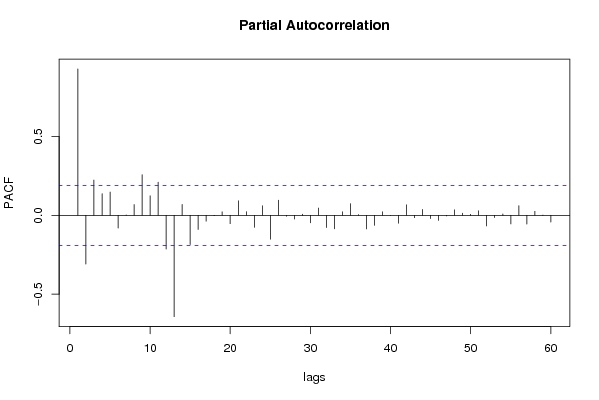
Title produced by software

(Partial) Autocorrelation Function

Date of computation

Tue, 23 Dec 2008 08:13:44 -0700

Cite this page as follows

Statistical Computations at FreeStatistics.org, Office for Research Development and Education, URL https://freestatistics.org/blog/index.php?v=date/2008/Dec/23/t1230045279qjjdkbsg7p76u6i.htm/, Retrieved Sun, 19 May 2024 10:44:54 +0000

Statistical Computations at FreeStatistics.org, Office for Research Development and Education, URL https://freestatistics.org/blog/index.php?pk=36316, Retrieved Sun, 19 May 2024 10:44:54 +0000

QR Codes:

Paste this QR Code to cite your computation.

Original text written by user:

IsPrivate?

No (this computation is public)

User-defined keywords

Estimated Impact

163

Family? (F = Feedback message, R = changed R code, M = changed R Module, P = changed Parameters, D = changed Data)

-     [Univariate Data Series] [data set] [2008-12-01 19:54:57] [b98453cac15ba1066b407e146608df68]
F RMP   [Standard Deviation-Mean Plot] [Q1 ] [2008-12-07 13:13:15] [74be16979710d4c4e7c6647856088456]
-    D    [Standard Deviation-Mean Plot] [SMP eigen tijdreeks] [2008-12-15 19:50:53] [74be16979710d4c4e7c6647856088456]
- RMPD      [(Partial) Autocorrelation Function] [paper] [2008-12-23 14:27:57] [5262baed313b307078ce11eb68e9efe6]
-   P         [(Partial) Autocorrelation Function] [paper] [2008-12-23 14:38:06] [5262baed313b307078ce11eb68e9efe6]
-   P             [(Partial) Autocorrelation Function] [Paper] [2008-12-23 15:13:44] [5bd06487453d0eec7a1bf04bf9f25085] [Current]
-   P               [(Partial) Autocorrelation Function] [paper] [2008-12-23 15:16:02] [5262baed313b307078ce11eb68e9efe6] 

Feedback Forum

Post a new message

Dataseries X:

Download CSV

Histogram

Boxplots

Summary of computational transaction
Raw Input	view raw input (R code)
Raw Output	view raw output of R engine
Computing time	1 seconds
R Server	'George Udny Yule' @ 72.249.76.132

\begin{tabular}{lllllllll}
\hline
Summary of computational transaction \tabularnewline
Raw Input & view raw input (R code)  \tabularnewline
Raw Output & view raw output of R engine  \tabularnewline
Computing time & 1 seconds \tabularnewline
R Server & 'George Udny Yule' @ 72.249.76.132 \tabularnewline
\hline
\end{tabular}
%Source: https://freestatistics.org/blog/index.php?pk=36316&T=0

[TABLE]
[ROW][C]Summary of computational transaction[/C][/ROW]
[ROW][C]Raw Input[/C][C]view raw input (R code) [/C][/ROW]
[ROW][C]Raw Output[/C][C]view raw output of R engine [/C][/ROW]
[ROW][C]Computing time[/C][C]1 seconds[/C][/ROW]
[ROW][C]R Server[/C][C]'George Udny Yule' @ 72.249.76.132[/C][/ROW]
[/TABLE]
Source: https://freestatistics.org/blog/index.php?pk=36316&T=0

Globally Unique Identifier (entire table): ba.freestatistics.org/blog/index.php?pk=36316&T=0

As an alternative you can also use a QR Code:

The GUIDs for individual cells are displayed in the table below:

Summary of computational transaction
Raw Input	view raw input (R code)
Raw Output	view raw output of R engine
Computing time	1 seconds
R Server	'George Udny Yule' @ 72.249.76.132

Autocorrelation Function
Time lag k	ACF(k)	T-STAT	P-value
1	0.928959	9.5642	0
2	0.820549	8.4481	0
3	0.738355	7.6018	0
4	0.696009	7.1659	0
5	0.686315	7.066	0
6	0.671491	6.9134	0
7	0.638973	6.5786	0
8	0.604692	6.2257	0
9	0.604312	6.2218	0
10	0.637382	6.5622	0
11	0.690451	7.1086	0
12	0.705429	7.2628	0
13	0.613949	6.321	0
14	0.496009	5.1067	1e-06
15	0.39847	4.1025	4e-05
16	0.336307	3.4625	0.000386
17	0.303495	3.1247	0.001148
18	0.268154	2.7608	0.003398
19	0.221225	2.2776	0.012377
20	0.174761	1.7993	0.03741
21	0.164613	1.6948	0.046526
22	0.186233	1.9174	0.02894
23	0.218749	2.2522	0.013187
24	0.2165	2.229	0.013962
25	0.128083	1.3187	0.095057
26	0.024515	0.2524	0.400611
27	-0.05742	-0.5912	0.27783
28	-0.107816	-1.11	0.134747
29	-0.134455	-1.3843	0.084587
30	-0.164494	-1.6936	0.046642
31	-0.200843	-2.0678	0.020546
32	-0.235491	-2.4245	0.00851
33	-0.238194	-2.4524	0.007912
34	-0.213784	-2.201	0.014951
35	-0.175983	-1.8119	0.03642
36	-0.167446	-1.724	0.043815
37	-0.233404	-2.403	0.008999
38	-0.31454	-3.2384	0.000803
39	-0.375929	-3.8704	9.4e-05
40	-0.404201	-4.1615	3.2e-05
41	-0.41269	-4.2489	2.3e-05
42	-0.422524	-4.3501	1.6e-05
43	-0.436498	-4.494	9e-06
44	-0.448325	-4.6158	6e-06
45	-0.432459	-4.4524	1.1e-05
46	-0.395314	-4.07	4.5e-05
47	-0.348096	-3.5839	0.000257
48	-0.323499	-3.3306	0.000597
49	-0.359393	-3.7002	0.000172
50	-0.408214	-4.2028	2.8e-05
51	-0.439679	-4.5268	8e-06
52	-0.446924	-4.6014	6e-06
53	-0.439155	-4.5214	8e-06
54	-0.429729	-4.4243	1.2e-05
55	-0.424497	-4.3705	1.5e-05
56	-0.415805	-4.281	2e-05
57	-0.383713	-3.9506	7e-05
58	-0.334839	-3.4474	0.000406
59	-0.278413	-2.8664	0.002504
60	-0.244841	-2.5208	0.006599

\begin{tabular}{lllllllll}
\hline
Autocorrelation Function \tabularnewline
Time lag k & ACF(k) & T-STAT & P-value \tabularnewline
1 & 0.928959 & 9.5642 & 0 \tabularnewline
2 & 0.820549 & 8.4481 & 0 \tabularnewline
3 & 0.738355 & 7.6018 & 0 \tabularnewline
4 & 0.696009 & 7.1659 & 0 \tabularnewline
5 & 0.686315 & 7.066 & 0 \tabularnewline
6 & 0.671491 & 6.9134 & 0 \tabularnewline
7 & 0.638973 & 6.5786 & 0 \tabularnewline
8 & 0.604692 & 6.2257 & 0 \tabularnewline
9 & 0.604312 & 6.2218 & 0 \tabularnewline
10 & 0.637382 & 6.5622 & 0 \tabularnewline
11 & 0.690451 & 7.1086 & 0 \tabularnewline
12 & 0.705429 & 7.2628 & 0 \tabularnewline
13 & 0.613949 & 6.321 & 0 \tabularnewline
14 & 0.496009 & 5.1067 & 1e-06 \tabularnewline
15 & 0.39847 & 4.1025 & 4e-05 \tabularnewline
16 & 0.336307 & 3.4625 & 0.000386 \tabularnewline
17 & 0.303495 & 3.1247 & 0.001148 \tabularnewline
18 & 0.268154 & 2.7608 & 0.003398 \tabularnewline
19 & 0.221225 & 2.2776 & 0.012377 \tabularnewline
20 & 0.174761 & 1.7993 & 0.03741 \tabularnewline
21 & 0.164613 & 1.6948 & 0.046526 \tabularnewline
22 & 0.186233 & 1.9174 & 0.02894 \tabularnewline
23 & 0.218749 & 2.2522 & 0.013187 \tabularnewline
24 & 0.2165 & 2.229 & 0.013962 \tabularnewline
25 & 0.128083 & 1.3187 & 0.095057 \tabularnewline
26 & 0.024515 & 0.2524 & 0.400611 \tabularnewline
27 & -0.05742 & -0.5912 & 0.27783 \tabularnewline
28 & -0.107816 & -1.11 & 0.134747 \tabularnewline
29 & -0.134455 & -1.3843 & 0.084587 \tabularnewline
30 & -0.164494 & -1.6936 & 0.046642 \tabularnewline
31 & -0.200843 & -2.0678 & 0.020546 \tabularnewline
32 & -0.235491 & -2.4245 & 0.00851 \tabularnewline
33 & -0.238194 & -2.4524 & 0.007912 \tabularnewline
34 & -0.213784 & -2.201 & 0.014951 \tabularnewline
35 & -0.175983 & -1.8119 & 0.03642 \tabularnewline
36 & -0.167446 & -1.724 & 0.043815 \tabularnewline
37 & -0.233404 & -2.403 & 0.008999 \tabularnewline
38 & -0.31454 & -3.2384 & 0.000803 \tabularnewline
39 & -0.375929 & -3.8704 & 9.4e-05 \tabularnewline
40 & -0.404201 & -4.1615 & 3.2e-05 \tabularnewline
41 & -0.41269 & -4.2489 & 2.3e-05 \tabularnewline
42 & -0.422524 & -4.3501 & 1.6e-05 \tabularnewline
43 & -0.436498 & -4.494 & 9e-06 \tabularnewline
44 & -0.448325 & -4.6158 & 6e-06 \tabularnewline
45 & -0.432459 & -4.4524 & 1.1e-05 \tabularnewline
46 & -0.395314 & -4.07 & 4.5e-05 \tabularnewline
47 & -0.348096 & -3.5839 & 0.000257 \tabularnewline
48 & -0.323499 & -3.3306 & 0.000597 \tabularnewline
49 & -0.359393 & -3.7002 & 0.000172 \tabularnewline
50 & -0.408214 & -4.2028 & 2.8e-05 \tabularnewline
51 & -0.439679 & -4.5268 & 8e-06 \tabularnewline
52 & -0.446924 & -4.6014 & 6e-06 \tabularnewline
53 & -0.439155 & -4.5214 & 8e-06 \tabularnewline
54 & -0.429729 & -4.4243 & 1.2e-05 \tabularnewline
55 & -0.424497 & -4.3705 & 1.5e-05 \tabularnewline
56 & -0.415805 & -4.281 & 2e-05 \tabularnewline
57 & -0.383713 & -3.9506 & 7e-05 \tabularnewline
58 & -0.334839 & -3.4474 & 0.000406 \tabularnewline
59 & -0.278413 & -2.8664 & 0.002504 \tabularnewline
60 & -0.244841 & -2.5208 & 0.006599 \tabularnewline
\hline
\end{tabular}
%Source: https://freestatistics.org/blog/index.php?pk=36316&T=1

[TABLE]
[ROW][C]Autocorrelation Function[/C][/ROW]
[ROW][C]Time lag k[/C][C]ACF(k)[/C][C]T-STAT[/C][C]P-value[/C][/ROW]
[ROW][C]1[/C][C]0.928959[/C][C]9.5642[/C][C]0[/C][/ROW]
[ROW][C]2[/C][C]0.820549[/C][C]8.4481[/C][C]0[/C][/ROW]
[ROW][C]3[/C][C]0.738355[/C][C]7.6018[/C][C]0[/C][/ROW]
[ROW][C]4[/C][C]0.696009[/C][C]7.1659[/C][C]0[/C][/ROW]
[ROW][C]5[/C][C]0.686315[/C][C]7.066[/C][C]0[/C][/ROW]
[ROW][C]6[/C][C]0.671491[/C][C]6.9134[/C][C]0[/C][/ROW]
[ROW][C]7[/C][C]0.638973[/C][C]6.5786[/C][C]0[/C][/ROW]
[ROW][C]8[/C][C]0.604692[/C][C]6.2257[/C][C]0[/C][/ROW]
[ROW][C]9[/C][C]0.604312[/C][C]6.2218[/C][C]0[/C][/ROW]
[ROW][C]10[/C][C]0.637382[/C][C]6.5622[/C][C]0[/C][/ROW]
[ROW][C]11[/C][C]0.690451[/C][C]7.1086[/C][C]0[/C][/ROW]
[ROW][C]12[/C][C]0.705429[/C][C]7.2628[/C][C]0[/C][/ROW]
[ROW][C]13[/C][C]0.613949[/C][C]6.321[/C][C]0[/C][/ROW]
[ROW][C]14[/C][C]0.496009[/C][C]5.1067[/C][C]1e-06[/C][/ROW]
[ROW][C]15[/C][C]0.39847[/C][C]4.1025[/C][C]4e-05[/C][/ROW]
[ROW][C]16[/C][C]0.336307[/C][C]3.4625[/C][C]0.000386[/C][/ROW]
[ROW][C]17[/C][C]0.303495[/C][C]3.1247[/C][C]0.001148[/C][/ROW]
[ROW][C]18[/C][C]0.268154[/C][C]2.7608[/C][C]0.003398[/C][/ROW]
[ROW][C]19[/C][C]0.221225[/C][C]2.2776[/C][C]0.012377[/C][/ROW]
[ROW][C]20[/C][C]0.174761[/C][C]1.7993[/C][C]0.03741[/C][/ROW]
[ROW][C]21[/C][C]0.164613[/C][C]1.6948[/C][C]0.046526[/C][/ROW]
[ROW][C]22[/C][C]0.186233[/C][C]1.9174[/C][C]0.02894[/C][/ROW]
[ROW][C]23[/C][C]0.218749[/C][C]2.2522[/C][C]0.013187[/C][/ROW]
[ROW][C]24[/C][C]0.2165[/C][C]2.229[/C][C]0.013962[/C][/ROW]
[ROW][C]25[/C][C]0.128083[/C][C]1.3187[/C][C]0.095057[/C][/ROW]
[ROW][C]26[/C][C]0.024515[/C][C]0.2524[/C][C]0.400611[/C][/ROW]
[ROW][C]27[/C][C]-0.05742[/C][C]-0.5912[/C][C]0.27783[/C][/ROW]
[ROW][C]28[/C][C]-0.107816[/C][C]-1.11[/C][C]0.134747[/C][/ROW]
[ROW][C]29[/C][C]-0.134455[/C][C]-1.3843[/C][C]0.084587[/C][/ROW]
[ROW][C]30[/C][C]-0.164494[/C][C]-1.6936[/C][C]0.046642[/C][/ROW]
[ROW][C]31[/C][C]-0.200843[/C][C]-2.0678[/C][C]0.020546[/C][/ROW]
[ROW][C]32[/C][C]-0.235491[/C][C]-2.4245[/C][C]0.00851[/C][/ROW]
[ROW][C]33[/C][C]-0.238194[/C][C]-2.4524[/C][C]0.007912[/C][/ROW]
[ROW][C]34[/C][C]-0.213784[/C][C]-2.201[/C][C]0.014951[/C][/ROW]
[ROW][C]35[/C][C]-0.175983[/C][C]-1.8119[/C][C]0.03642[/C][/ROW]
[ROW][C]36[/C][C]-0.167446[/C][C]-1.724[/C][C]0.043815[/C][/ROW]
[ROW][C]37[/C][C]-0.233404[/C][C]-2.403[/C][C]0.008999[/C][/ROW]
[ROW][C]38[/C][C]-0.31454[/C][C]-3.2384[/C][C]0.000803[/C][/ROW]
[ROW][C]39[/C][C]-0.375929[/C][C]-3.8704[/C][C]9.4e-05[/C][/ROW]
[ROW][C]40[/C][C]-0.404201[/C][C]-4.1615[/C][C]3.2e-05[/C][/ROW]
[ROW][C]41[/C][C]-0.41269[/C][C]-4.2489[/C][C]2.3e-05[/C][/ROW]
[ROW][C]42[/C][C]-0.422524[/C][C]-4.3501[/C][C]1.6e-05[/C][/ROW]
[ROW][C]43[/C][C]-0.436498[/C][C]-4.494[/C][C]9e-06[/C][/ROW]
[ROW][C]44[/C][C]-0.448325[/C][C]-4.6158[/C][C]6e-06[/C][/ROW]
[ROW][C]45[/C][C]-0.432459[/C][C]-4.4524[/C][C]1.1e-05[/C][/ROW]
[ROW][C]46[/C][C]-0.395314[/C][C]-4.07[/C][C]4.5e-05[/C][/ROW]
[ROW][C]47[/C][C]-0.348096[/C][C]-3.5839[/C][C]0.000257[/C][/ROW]
[ROW][C]48[/C][C]-0.323499[/C][C]-3.3306[/C][C]0.000597[/C][/ROW]
[ROW][C]49[/C][C]-0.359393[/C][C]-3.7002[/C][C]0.000172[/C][/ROW]
[ROW][C]50[/C][C]-0.408214[/C][C]-4.2028[/C][C]2.8e-05[/C][/ROW]
[ROW][C]51[/C][C]-0.439679[/C][C]-4.5268[/C][C]8e-06[/C][/ROW]
[ROW][C]52[/C][C]-0.446924[/C][C]-4.6014[/C][C]6e-06[/C][/ROW]
[ROW][C]53[/C][C]-0.439155[/C][C]-4.5214[/C][C]8e-06[/C][/ROW]
[ROW][C]54[/C][C]-0.429729[/C][C]-4.4243[/C][C]1.2e-05[/C][/ROW]
[ROW][C]55[/C][C]-0.424497[/C][C]-4.3705[/C][C]1.5e-05[/C][/ROW]
[ROW][C]56[/C][C]-0.415805[/C][C]-4.281[/C][C]2e-05[/C][/ROW]
[ROW][C]57[/C][C]-0.383713[/C][C]-3.9506[/C][C]7e-05[/C][/ROW]
[ROW][C]58[/C][C]-0.334839[/C][C]-3.4474[/C][C]0.000406[/C][/ROW]
[ROW][C]59[/C][C]-0.278413[/C][C]-2.8664[/C][C]0.002504[/C][/ROW]
[ROW][C]60[/C][C]-0.244841[/C][C]-2.5208[/C][C]0.006599[/C][/ROW]
[/TABLE]
Source: https://freestatistics.org/blog/index.php?pk=36316&T=1

Globally Unique Identifier (entire table): ba.freestatistics.org/blog/index.php?pk=36316&T=1

As an alternative you can also use a QR Code:

The GUIDs for individual cells are displayed in the table below:

Autocorrelation Function
Time lag k	ACF(k)	T-STAT	P-value
1	0.928959	9.5642	0
2	0.820549	8.4481	0
3	0.738355	7.6018	0
4	0.696009	7.1659	0
5	0.686315	7.066	0
6	0.671491	6.9134	0
7	0.638973	6.5786	0
8	0.604692	6.2257	0
9	0.604312	6.2218	0
10	0.637382	6.5622	0
11	0.690451	7.1086	0
12	0.705429	7.2628	0
13	0.613949	6.321	0
14	0.496009	5.1067	1e-06
15	0.39847	4.1025	4e-05
16	0.336307	3.4625	0.000386
17	0.303495	3.1247	0.001148
18	0.268154	2.7608	0.003398
19	0.221225	2.2776	0.012377
20	0.174761	1.7993	0.03741
21	0.164613	1.6948	0.046526
22	0.186233	1.9174	0.02894
23	0.218749	2.2522	0.013187
24	0.2165	2.229	0.013962
25	0.128083	1.3187	0.095057
26	0.024515	0.2524	0.400611
27	-0.05742	-0.5912	0.27783
28	-0.107816	-1.11	0.134747
29	-0.134455	-1.3843	0.084587
30	-0.164494	-1.6936	0.046642
31	-0.200843	-2.0678	0.020546
32	-0.235491	-2.4245	0.00851
33	-0.238194	-2.4524	0.007912
34	-0.213784	-2.201	0.014951
35	-0.175983	-1.8119	0.03642
36	-0.167446	-1.724	0.043815
37	-0.233404	-2.403	0.008999
38	-0.31454	-3.2384	0.000803
39	-0.375929	-3.8704	9.4e-05
40	-0.404201	-4.1615	3.2e-05
41	-0.41269	-4.2489	2.3e-05
42	-0.422524	-4.3501	1.6e-05
43	-0.436498	-4.494	9e-06
44	-0.448325	-4.6158	6e-06
45	-0.432459	-4.4524	1.1e-05
46	-0.395314	-4.07	4.5e-05
47	-0.348096	-3.5839	0.000257
48	-0.323499	-3.3306	0.000597
49	-0.359393	-3.7002	0.000172
50	-0.408214	-4.2028	2.8e-05
51	-0.439679	-4.5268	8e-06
52	-0.446924	-4.6014	6e-06
53	-0.439155	-4.5214	8e-06
54	-0.429729	-4.4243	1.2e-05
55	-0.424497	-4.3705	1.5e-05
56	-0.415805	-4.281	2e-05
57	-0.383713	-3.9506	7e-05
58	-0.334839	-3.4474	0.000406
59	-0.278413	-2.8664	0.002504
60	-0.244841	-2.5208	0.006599

Partial Autocorrelation Function
Time lag k	PACF(k)	T-STAT	P-value
1	0.928959	9.5642	0
2	-0.309535	-3.1869	0.000945
3	0.223547	2.3016	0.011658
4	0.137399	1.4146	0.080057
5	0.14777	1.5214	0.065571
6	-0.081024	-0.8342	0.203025
7	0.002745	0.0283	0.488752
8	0.06824	0.7026	0.24193
9	0.257595	2.6521	0.004614
10	0.123664	1.2732	0.102866
11	0.210467	2.1669	0.016241
12	-0.214213	-2.2055	0.014791
13	-0.642938	-6.6195	0
14	0.069022	0.7106	0.23944
15	-0.185379	-1.9086	0.02951
16	-0.089609	-0.9226	0.179161
17	-0.036958	-0.3805	0.352167
18	-0.001882	-0.0194	0.492289
19	0.022354	0.2302	0.409208
20	-0.052809	-0.5437	0.293893
21	0.092041	0.9476	0.172739
22	0.023341	0.2403	0.405278
23	-0.076329	-0.7859	0.216852
24	0.060677	0.6247	0.266753
25	-0.151602	-1.5608	0.060771
26	0.096391	0.9924	0.16163
27	-0.005667	-0.0583	0.476793
28	-0.023414	-0.2411	0.404987
29	0.007067	0.0728	0.471067
30	-0.047649	-0.4906	0.312371
31	0.046006	0.4737	0.318358
32	-0.077902	-0.8021	0.212159
33	-0.085787	-0.8832	0.189555
34	0.022775	0.2345	0.407533
35	0.073684	0.7586	0.22488
36	0.00512	0.0527	0.479029
37	-0.086678	-0.8924	0.187099
38	-0.063327	-0.652	0.257908
39	0.022158	0.2281	0.409993
40	-0.000223	-0.0023	0.499086
41	-0.050203	-0.5169	0.303161
42	0.066731	0.687	0.246781
43	-0.015173	-0.1562	0.438081
44	0.037733	0.3885	0.34922
45	-0.020827	-0.2144	0.415314
46	-0.032085	-0.3303	0.3709
47	-0.003502	-0.0361	0.485653
48	0.035212	0.3625	0.358841
49	0.013801	0.1421	0.443639
50	0.006894	0.071	0.471773
51	0.028918	0.2977	0.383246
52	-0.066962	-0.6894	0.246035
53	-0.014124	-0.1454	0.44233
54	0.008856	0.0912	0.463762
55	-0.054435	-0.5604	0.28818
56	0.060955	0.6276	0.265818
57	-0.055615	-0.5726	0.284066
58	0.025879	0.2664	0.395208
59	0.001562	0.0161	0.493599
60	-0.042936	-0.4421	0.329674

\begin{tabular}{lllllllll}
\hline
Partial Autocorrelation Function \tabularnewline
Time lag k & PACF(k) & T-STAT & P-value \tabularnewline
1 & 0.928959 & 9.5642 & 0 \tabularnewline
2 & -0.309535 & -3.1869 & 0.000945 \tabularnewline
3 & 0.223547 & 2.3016 & 0.011658 \tabularnewline
4 & 0.137399 & 1.4146 & 0.080057 \tabularnewline
5 & 0.14777 & 1.5214 & 0.065571 \tabularnewline
6 & -0.081024 & -0.8342 & 0.203025 \tabularnewline
7 & 0.002745 & 0.0283 & 0.488752 \tabularnewline
8 & 0.06824 & 0.7026 & 0.24193 \tabularnewline
9 & 0.257595 & 2.6521 & 0.004614 \tabularnewline
10 & 0.123664 & 1.2732 & 0.102866 \tabularnewline
11 & 0.210467 & 2.1669 & 0.016241 \tabularnewline
12 & -0.214213 & -2.2055 & 0.014791 \tabularnewline
13 & -0.642938 & -6.6195 & 0 \tabularnewline
14 & 0.069022 & 0.7106 & 0.23944 \tabularnewline
15 & -0.185379 & -1.9086 & 0.02951 \tabularnewline
16 & -0.089609 & -0.9226 & 0.179161 \tabularnewline
17 & -0.036958 & -0.3805 & 0.352167 \tabularnewline
18 & -0.001882 & -0.0194 & 0.492289 \tabularnewline
19 & 0.022354 & 0.2302 & 0.409208 \tabularnewline
20 & -0.052809 & -0.5437 & 0.293893 \tabularnewline
21 & 0.092041 & 0.9476 & 0.172739 \tabularnewline
22 & 0.023341 & 0.2403 & 0.405278 \tabularnewline
23 & -0.076329 & -0.7859 & 0.216852 \tabularnewline
24 & 0.060677 & 0.6247 & 0.266753 \tabularnewline
25 & -0.151602 & -1.5608 & 0.060771 \tabularnewline
26 & 0.096391 & 0.9924 & 0.16163 \tabularnewline
27 & -0.005667 & -0.0583 & 0.476793 \tabularnewline
28 & -0.023414 & -0.2411 & 0.404987 \tabularnewline
29 & 0.007067 & 0.0728 & 0.471067 \tabularnewline
30 & -0.047649 & -0.4906 & 0.312371 \tabularnewline
31 & 0.046006 & 0.4737 & 0.318358 \tabularnewline
32 & -0.077902 & -0.8021 & 0.212159 \tabularnewline
33 & -0.085787 & -0.8832 & 0.189555 \tabularnewline
34 & 0.022775 & 0.2345 & 0.407533 \tabularnewline
35 & 0.073684 & 0.7586 & 0.22488 \tabularnewline
36 & 0.00512 & 0.0527 & 0.479029 \tabularnewline
37 & -0.086678 & -0.8924 & 0.187099 \tabularnewline
38 & -0.063327 & -0.652 & 0.257908 \tabularnewline
39 & 0.022158 & 0.2281 & 0.409993 \tabularnewline
40 & -0.000223 & -0.0023 & 0.499086 \tabularnewline
41 & -0.050203 & -0.5169 & 0.303161 \tabularnewline
42 & 0.066731 & 0.687 & 0.246781 \tabularnewline
43 & -0.015173 & -0.1562 & 0.438081 \tabularnewline
44 & 0.037733 & 0.3885 & 0.34922 \tabularnewline
45 & -0.020827 & -0.2144 & 0.415314 \tabularnewline
46 & -0.032085 & -0.3303 & 0.3709 \tabularnewline
47 & -0.003502 & -0.0361 & 0.485653 \tabularnewline
48 & 0.035212 & 0.3625 & 0.358841 \tabularnewline
49 & 0.013801 & 0.1421 & 0.443639 \tabularnewline
50 & 0.006894 & 0.071 & 0.471773 \tabularnewline
51 & 0.028918 & 0.2977 & 0.383246 \tabularnewline
52 & -0.066962 & -0.6894 & 0.246035 \tabularnewline
53 & -0.014124 & -0.1454 & 0.44233 \tabularnewline
54 & 0.008856 & 0.0912 & 0.463762 \tabularnewline
55 & -0.054435 & -0.5604 & 0.28818 \tabularnewline
56 & 0.060955 & 0.6276 & 0.265818 \tabularnewline
57 & -0.055615 & -0.5726 & 0.284066 \tabularnewline
58 & 0.025879 & 0.2664 & 0.395208 \tabularnewline
59 & 0.001562 & 0.0161 & 0.493599 \tabularnewline
60 & -0.042936 & -0.4421 & 0.329674 \tabularnewline
\hline
\end{tabular}
%Source: https://freestatistics.org/blog/index.php?pk=36316&T=2

[TABLE]
[ROW][C]Partial Autocorrelation Function[/C][/ROW]
[ROW][C]Time lag k[/C][C]PACF(k)[/C][C]T-STAT[/C][C]P-value[/C][/ROW]
[ROW][C]1[/C][C]0.928959[/C][C]9.5642[/C][C]0[/C][/ROW]
[ROW][C]2[/C][C]-0.309535[/C][C]-3.1869[/C][C]0.000945[/C][/ROW]
[ROW][C]3[/C][C]0.223547[/C][C]2.3016[/C][C]0.011658[/C][/ROW]
[ROW][C]4[/C][C]0.137399[/C][C]1.4146[/C][C]0.080057[/C][/ROW]
[ROW][C]5[/C][C]0.14777[/C][C]1.5214[/C][C]0.065571[/C][/ROW]
[ROW][C]6[/C][C]-0.081024[/C][C]-0.8342[/C][C]0.203025[/C][/ROW]
[ROW][C]7[/C][C]0.002745[/C][C]0.0283[/C][C]0.488752[/C][/ROW]
[ROW][C]8[/C][C]0.06824[/C][C]0.7026[/C][C]0.24193[/C][/ROW]
[ROW][C]9[/C][C]0.257595[/C][C]2.6521[/C][C]0.004614[/C][/ROW]
[ROW][C]10[/C][C]0.123664[/C][C]1.2732[/C][C]0.102866[/C][/ROW]
[ROW][C]11[/C][C]0.210467[/C][C]2.1669[/C][C]0.016241[/C][/ROW]
[ROW][C]12[/C][C]-0.214213[/C][C]-2.2055[/C][C]0.014791[/C][/ROW]
[ROW][C]13[/C][C]-0.642938[/C][C]-6.6195[/C][C]0[/C][/ROW]
[ROW][C]14[/C][C]0.069022[/C][C]0.7106[/C][C]0.23944[/C][/ROW]
[ROW][C]15[/C][C]-0.185379[/C][C]-1.9086[/C][C]0.02951[/C][/ROW]
[ROW][C]16[/C][C]-0.089609[/C][C]-0.9226[/C][C]0.179161[/C][/ROW]
[ROW][C]17[/C][C]-0.036958[/C][C]-0.3805[/C][C]0.352167[/C][/ROW]
[ROW][C]18[/C][C]-0.001882[/C][C]-0.0194[/C][C]0.492289[/C][/ROW]
[ROW][C]19[/C][C]0.022354[/C][C]0.2302[/C][C]0.409208[/C][/ROW]
[ROW][C]20[/C][C]-0.052809[/C][C]-0.5437[/C][C]0.293893[/C][/ROW]
[ROW][C]21[/C][C]0.092041[/C][C]0.9476[/C][C]0.172739[/C][/ROW]
[ROW][C]22[/C][C]0.023341[/C][C]0.2403[/C][C]0.405278[/C][/ROW]
[ROW][C]23[/C][C]-0.076329[/C][C]-0.7859[/C][C]0.216852[/C][/ROW]
[ROW][C]24[/C][C]0.060677[/C][C]0.6247[/C][C]0.266753[/C][/ROW]
[ROW][C]25[/C][C]-0.151602[/C][C]-1.5608[/C][C]0.060771[/C][/ROW]
[ROW][C]26[/C][C]0.096391[/C][C]0.9924[/C][C]0.16163[/C][/ROW]
[ROW][C]27[/C][C]-0.005667[/C][C]-0.0583[/C][C]0.476793[/C][/ROW]
[ROW][C]28[/C][C]-0.023414[/C][C]-0.2411[/C][C]0.404987[/C][/ROW]
[ROW][C]29[/C][C]0.007067[/C][C]0.0728[/C][C]0.471067[/C][/ROW]
[ROW][C]30[/C][C]-0.047649[/C][C]-0.4906[/C][C]0.312371[/C][/ROW]
[ROW][C]31[/C][C]0.046006[/C][C]0.4737[/C][C]0.318358[/C][/ROW]
[ROW][C]32[/C][C]-0.077902[/C][C]-0.8021[/C][C]0.212159[/C][/ROW]
[ROW][C]33[/C][C]-0.085787[/C][C]-0.8832[/C][C]0.189555[/C][/ROW]
[ROW][C]34[/C][C]0.022775[/C][C]0.2345[/C][C]0.407533[/C][/ROW]
[ROW][C]35[/C][C]0.073684[/C][C]0.7586[/C][C]0.22488[/C][/ROW]
[ROW][C]36[/C][C]0.00512[/C][C]0.0527[/C][C]0.479029[/C][/ROW]
[ROW][C]37[/C][C]-0.086678[/C][C]-0.8924[/C][C]0.187099[/C][/ROW]
[ROW][C]38[/C][C]-0.063327[/C][C]-0.652[/C][C]0.257908[/C][/ROW]
[ROW][C]39[/C][C]0.022158[/C][C]0.2281[/C][C]0.409993[/C][/ROW]
[ROW][C]40[/C][C]-0.000223[/C][C]-0.0023[/C][C]0.499086[/C][/ROW]
[ROW][C]41[/C][C]-0.050203[/C][C]-0.5169[/C][C]0.303161[/C][/ROW]
[ROW][C]42[/C][C]0.066731[/C][C]0.687[/C][C]0.246781[/C][/ROW]
[ROW][C]43[/C][C]-0.015173[/C][C]-0.1562[/C][C]0.438081[/C][/ROW]
[ROW][C]44[/C][C]0.037733[/C][C]0.3885[/C][C]0.34922[/C][/ROW]
[ROW][C]45[/C][C]-0.020827[/C][C]-0.2144[/C][C]0.415314[/C][/ROW]
[ROW][C]46[/C][C]-0.032085[/C][C]-0.3303[/C][C]0.3709[/C][/ROW]
[ROW][C]47[/C][C]-0.003502[/C][C]-0.0361[/C][C]0.485653[/C][/ROW]
[ROW][C]48[/C][C]0.035212[/C][C]0.3625[/C][C]0.358841[/C][/ROW]
[ROW][C]49[/C][C]0.013801[/C][C]0.1421[/C][C]0.443639[/C][/ROW]
[ROW][C]50[/C][C]0.006894[/C][C]0.071[/C][C]0.471773[/C][/ROW]
[ROW][C]51[/C][C]0.028918[/C][C]0.2977[/C][C]0.383246[/C][/ROW]
[ROW][C]52[/C][C]-0.066962[/C][C]-0.6894[/C][C]0.246035[/C][/ROW]
[ROW][C]53[/C][C]-0.014124[/C][C]-0.1454[/C][C]0.44233[/C][/ROW]
[ROW][C]54[/C][C]0.008856[/C][C]0.0912[/C][C]0.463762[/C][/ROW]
[ROW][C]55[/C][C]-0.054435[/C][C]-0.5604[/C][C]0.28818[/C][/ROW]
[ROW][C]56[/C][C]0.060955[/C][C]0.6276[/C][C]0.265818[/C][/ROW]
[ROW][C]57[/C][C]-0.055615[/C][C]-0.5726[/C][C]0.284066[/C][/ROW]
[ROW][C]58[/C][C]0.025879[/C][C]0.2664[/C][C]0.395208[/C][/ROW]
[ROW][C]59[/C][C]0.001562[/C][C]0.0161[/C][C]0.493599[/C][/ROW]
[ROW][C]60[/C][C]-0.042936[/C][C]-0.4421[/C][C]0.329674[/C][/ROW]
[/TABLE]
Source: https://freestatistics.org/blog/index.php?pk=36316&T=2

Globally Unique Identifier (entire table): ba.freestatistics.org/blog/index.php?pk=36316&T=2

As an alternative you can also use a QR Code:

The GUIDs for individual cells are displayed in the table below:

Partial Autocorrelation Function
Time lag k	PACF(k)	T-STAT	P-value
1	0.928959	9.5642	0
2	-0.309535	-3.1869	0.000945
3	0.223547	2.3016	0.011658
4	0.137399	1.4146	0.080057
5	0.14777	1.5214	0.065571
6	-0.081024	-0.8342	0.203025
7	0.002745	0.0283	0.488752
8	0.06824	0.7026	0.24193
9	0.257595	2.6521	0.004614
10	0.123664	1.2732	0.102866
11	0.210467	2.1669	0.016241
12	-0.214213	-2.2055	0.014791
13	-0.642938	-6.6195	0
14	0.069022	0.7106	0.23944
15	-0.185379	-1.9086	0.02951
16	-0.089609	-0.9226	0.179161
17	-0.036958	-0.3805	0.352167
18	-0.001882	-0.0194	0.492289
19	0.022354	0.2302	0.409208
20	-0.052809	-0.5437	0.293893
21	0.092041	0.9476	0.172739
22	0.023341	0.2403	0.405278
23	-0.076329	-0.7859	0.216852
24	0.060677	0.6247	0.266753
25	-0.151602	-1.5608	0.060771
26	0.096391	0.9924	0.16163
27	-0.005667	-0.0583	0.476793
28	-0.023414	-0.2411	0.404987
29	0.007067	0.0728	0.471067
30	-0.047649	-0.4906	0.312371
31	0.046006	0.4737	0.318358
32	-0.077902	-0.8021	0.212159
33	-0.085787	-0.8832	0.189555
34	0.022775	0.2345	0.407533
35	0.073684	0.7586	0.22488
36	0.00512	0.0527	0.479029
37	-0.086678	-0.8924	0.187099
38	-0.063327	-0.652	0.257908
39	0.022158	0.2281	0.409993
40	-0.000223	-0.0023	0.499086
41	-0.050203	-0.5169	0.303161
42	0.066731	0.687	0.246781
43	-0.015173	-0.1562	0.438081
44	0.037733	0.3885	0.34922
45	-0.020827	-0.2144	0.415314
46	-0.032085	-0.3303	0.3709
47	-0.003502	-0.0361	0.485653
48	0.035212	0.3625	0.358841
49	0.013801	0.1421	0.443639
50	0.006894	0.071	0.471773
51	0.028918	0.2977	0.383246
52	-0.066962	-0.6894	0.246035
53	-0.014124	-0.1454	0.44233
54	0.008856	0.0912	0.463762
55	-0.054435	-0.5604	0.28818
56	0.060955	0.6276	0.265818
57	-0.055615	-0.5726	0.284066
58	0.025879	0.2664	0.395208
59	0.001562	0.0161	0.493599
60	-0.042936	-0.4421	0.329674

Figure 1

PNG link

Postscript link

PDF link

Figure 2

PNG link

Postscript link

PDF link

Parameters (Session):

par1 = 60 ; par2 = 1 ; par3 = 0 ; par4 = 0 ; par5 = 12 ;

Parameters (R input):

par1 = 60 ; par2 = 1 ; par3 = 0 ; par4 = 0 ; par5 = 12 ;

R code (references can be found in the software module):

if (par1 == 'Default') {
par1 = 10*log10(length(x))
} else {
par1 <- as.numeric(par1)
}
par2 <- as.numeric(par2)
par3 <- as.numeric(par3)
par4 <- as.numeric(par4)
par5 <- as.numeric(par5)
if (par2 == 0) {
x <- log(x)
} else {
x <- (x ^ par2 - 1) / par2
}
if (par3 > 0) x <- diff(x,lag=1,difference=par3)
if (par4 > 0) x <- diff(x,lag=par5,difference=par4)
bitmap(file='pic1.png')
racf <- acf(x,par1,main='Autocorrelation',xlab='lags',ylab='ACF')
dev.off()
bitmap(file='pic2.png')
rpacf <- pacf(x,par1,main='Partial Autocorrelation',xlab='lags',ylab='PACF')
dev.off()
(myacf <- c(racf$acf))
(mypacf <- c(rpacf$acf))
lengthx <- length(x)
sqrtn <- sqrt(lengthx)
load(file='createtable')
a<-table.start()
a<-table.row.start(a)
a<-table.element(a,'Autocorrelation Function',4,TRUE)
a<-table.row.end(a)
a<-table.row.start(a)
a<-table.element(a,'Time lag k',header=TRUE)
a<-table.element(a,hyperlink('basics.htm','ACF(k)','click here for more information about the Autocorrelation Function'),header=TRUE)
a<-table.element(a,'T-STAT',header=TRUE)
a<-table.element(a,'P-value',header=TRUE)
a<-table.row.end(a)
for (i in 2:(par1+1)) {
a<-table.row.start(a)
a<-table.element(a,i-1,header=TRUE)
a<-table.element(a,round(myacf[i],6))
mytstat <- myacf[i]*sqrtn
a<-table.element(a,round(mytstat,4))
a<-table.element(a,round(1-pt(abs(mytstat),lengthx),6))
a<-table.row.end(a)
}
a<-table.end(a)
table.save(a,file='mytable.tab')
a<-table.start()
a<-table.row.start(a)
a<-table.element(a,'Partial Autocorrelation Function',4,TRUE)
a<-table.row.end(a)
a<-table.row.start(a)
a<-table.element(a,'Time lag k',header=TRUE)
a<-table.element(a,hyperlink('basics.htm','PACF(k)','click here for more information about the Partial Autocorrelation Function'),header=TRUE)
a<-table.element(a,'T-STAT',header=TRUE)
a<-table.element(a,'P-value',header=TRUE)
a<-table.row.end(a)
for (i in 1:par1) {
a<-table.row.start(a)
a<-table.element(a,i,header=TRUE)
a<-table.element(a,round(mypacf[i],6))
mytstat <- mypacf[i]*sqrtn
a<-table.element(a,round(mytstat,4))
a<-table.element(a,round(1-pt(abs(mytstat),lengthx),6))
a<-table.row.end(a)
}
a<-table.end(a)
table.save(a,file='mytable1.tab')

Free Statistics

Description of Statistical Computation

Tree of Dependent Computations

Dataset

Tables (Output of Computation)

Figures (Output of Computation)

Input Parameters & R Code