Repository of Reproducible Computations

Free Statistics

of Irreproducible Research!

Author's title

Author

*The author of this computation has been verified*

R Software Module

rwasp_autocorrelation.wasp

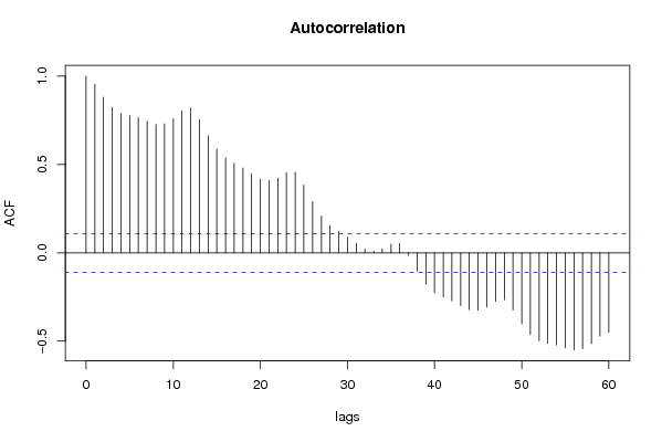
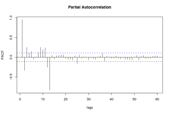
Title produced by software

(Partial) Autocorrelation Function

Date of computation

Sun, 21 Dec 2008 14:03:40 -0700

Cite this page as follows

Statistical Computations at FreeStatistics.org, Office for Research Development and Education, URL https://freestatistics.org/blog/index.php?v=date/2008/Dec/21/t12298935217dfnm0idkiq25r6.htm/, Retrieved Sun, 19 May 2024 09:25:58 +0000

Statistical Computations at FreeStatistics.org, Office for Research Development and Education, URL https://freestatistics.org/blog/index.php?pk=35827, Retrieved Sun, 19 May 2024 09:25:58 +0000

QR Codes:

Paste this QR Code to cite your computation.

Original text written by user:

IsPrivate?

No (this computation is public)

User-defined keywords

s0800650 Jan Werkhoven

Estimated Impact

203

Family? (F = Feedback message, R = changed R code, M = changed R Module, P = changed Parameters, D = changed Data)

-     [Univariate Data Series] [Werkloosheid: Tot...] [2008-11-03 21:02:03] [944cfe91fab3d898afdbc7f6b8914047]
- R PD  [Univariate Data Series] [Total unemployeme...] [2008-12-10 16:35:06] [944cfe91fab3d898afdbc7f6b8914047]
-   PD    [Univariate Data Series] [Total unemployeme...] [2008-12-10 18:49:43] [944cfe91fab3d898afdbc7f6b8914047]
- RMP         [(Partial) Autocorrelation Function] [D1: Autocorrelati...] [2008-12-21 21:03:40] [721fbc57bdc4e4e6ec78137fe5a723c9] [Current]
-    D          [(Partial) Autocorrelation Function] [400 random number...] [2008-12-21 21:08:32] [944cfe91fab3d898afdbc7f6b8914047] 

Feedback Forum

Post a new message

Dataseries X:

Download CSV

Histogram

Boxplots

Summary of computational transaction
Raw Input	view raw input (R code)
Raw Output	view raw output of R engine
Computing time	2 seconds
R Server	'Sir Ronald Aylmer Fisher' @ 193.190.124.24

\begin{tabular}{lllllllll}
\hline
Summary of computational transaction \tabularnewline
Raw Input & view raw input (R code)  \tabularnewline
Raw Output & view raw output of R engine  \tabularnewline
Computing time & 2 seconds \tabularnewline
R Server & 'Sir Ronald Aylmer Fisher' @ 193.190.124.24 \tabularnewline
\hline
\end{tabular}
%Source: https://freestatistics.org/blog/index.php?pk=35827&T=0

[TABLE]
[ROW][C]Summary of computational transaction[/C][/ROW]
[ROW][C]Raw Input[/C][C]view raw input (R code) [/C][/ROW]
[ROW][C]Raw Output[/C][C]view raw output of R engine [/C][/ROW]
[ROW][C]Computing time[/C][C]2 seconds[/C][/ROW]
[ROW][C]R Server[/C][C]'Sir Ronald Aylmer Fisher' @ 193.190.124.24[/C][/ROW]
[/TABLE]
Source: https://freestatistics.org/blog/index.php?pk=35827&T=0

Globally Unique Identifier (entire table): ba.freestatistics.org/blog/index.php?pk=35827&T=0

As an alternative you can also use a QR Code:

The GUIDs for individual cells are displayed in the table below:

Summary of computational transaction
Raw Input	view raw input (R code)
Raw Output	view raw output of R engine
Computing time	2 seconds
R Server	'Sir Ronald Aylmer Fisher' @ 193.190.124.24

Autocorrelation Function
Time lag k	ACF(k)	T-STAT	P-value
1	0.954318	17.1246	0
2	0.881011	15.8092	0
3	0.823093	14.7699	0
4	0.789259	14.1627	0
5	0.776395	13.9319	0
6	0.764867	13.7251	0
7	0.744763	13.3643	0
8	0.727002	13.0456	0
9	0.731164	13.1203	0
10	0.759437	13.6276	0
11	0.803195	14.4128	0
12	0.819522	14.7058	0
13	0.75413	13.5324	0
14	0.663154	11.8999	0
15	0.587386	10.5403	0
16	0.5368	9.6325	0
17	0.507751	9.1113	0
18	0.480966	8.6306	0
19	0.447285	8.0262	0
20	0.416913	7.4812	0
21	0.408294	7.3266	0
22	0.423297	7.5958	0
23	0.45275	8.1243	0
24	0.456126	8.1849	0
25	0.383912	6.8891	0
26	0.288419	5.1755	0
27	0.207873	3.7301	0.000113
28	0.153224	2.7495	0.003153
29	0.120446	2.1613	0.015704
30	0.089788	1.6112	0.054059
31	0.053486	0.9598	0.168946
32	0.021186	0.3802	0.352038
33	0.009904	0.1777	0.429528
34	0.021804	0.3913	0.34793
35	0.048504	0.8704	0.192374
36	0.051716	0.928	0.17705
37	-0.015754	-0.2827	0.388795
38	-0.104579	-1.8766	0.030738
39	-0.177919	-3.1926	0.000774
40	-0.224689	-4.0319	3.5e-05
41	-0.249561	-4.4782	5e-06
42	-0.271458	-4.8711	1e-06
43	-0.298489	-5.3562	0
44	-0.322191	-5.7815	0
45	-0.325641	-5.8434	0
46	-0.307477	-5.5175	0
47	-0.27537	-4.9413	1e-06
48	-0.266114	-4.7752	1e-06
49	-0.323988	-5.8138	0
50	-0.401756	-7.2093	0
51	-0.463211	-8.312	0
52	-0.498984	-8.9539	0
53	-0.513031	-9.206	0
54	-0.52272	-9.3799	0
55	-0.537486	-9.6448	0
56	-0.549477	-9.86	0
57	-0.54203	-9.7264	0
58	-0.513581	-9.2159	0
59	-0.471285	-8.4569	0
60	-0.450437	-8.0828	0

\begin{tabular}{lllllllll}
\hline
Autocorrelation Function \tabularnewline
Time lag k & ACF(k) & T-STAT & P-value \tabularnewline
1 & 0.954318 & 17.1246 & 0 \tabularnewline
2 & 0.881011 & 15.8092 & 0 \tabularnewline
3 & 0.823093 & 14.7699 & 0 \tabularnewline
4 & 0.789259 & 14.1627 & 0 \tabularnewline
5 & 0.776395 & 13.9319 & 0 \tabularnewline
6 & 0.764867 & 13.7251 & 0 \tabularnewline
7 & 0.744763 & 13.3643 & 0 \tabularnewline
8 & 0.727002 & 13.0456 & 0 \tabularnewline
9 & 0.731164 & 13.1203 & 0 \tabularnewline
10 & 0.759437 & 13.6276 & 0 \tabularnewline
11 & 0.803195 & 14.4128 & 0 \tabularnewline
12 & 0.819522 & 14.7058 & 0 \tabularnewline
13 & 0.75413 & 13.5324 & 0 \tabularnewline
14 & 0.663154 & 11.8999 & 0 \tabularnewline
15 & 0.587386 & 10.5403 & 0 \tabularnewline
16 & 0.5368 & 9.6325 & 0 \tabularnewline
17 & 0.507751 & 9.1113 & 0 \tabularnewline
18 & 0.480966 & 8.6306 & 0 \tabularnewline
19 & 0.447285 & 8.0262 & 0 \tabularnewline
20 & 0.416913 & 7.4812 & 0 \tabularnewline
21 & 0.408294 & 7.3266 & 0 \tabularnewline
22 & 0.423297 & 7.5958 & 0 \tabularnewline
23 & 0.45275 & 8.1243 & 0 \tabularnewline
24 & 0.456126 & 8.1849 & 0 \tabularnewline
25 & 0.383912 & 6.8891 & 0 \tabularnewline
26 & 0.288419 & 5.1755 & 0 \tabularnewline
27 & 0.207873 & 3.7301 & 0.000113 \tabularnewline
28 & 0.153224 & 2.7495 & 0.003153 \tabularnewline
29 & 0.120446 & 2.1613 & 0.015704 \tabularnewline
30 & 0.089788 & 1.6112 & 0.054059 \tabularnewline
31 & 0.053486 & 0.9598 & 0.168946 \tabularnewline
32 & 0.021186 & 0.3802 & 0.352038 \tabularnewline
33 & 0.009904 & 0.1777 & 0.429528 \tabularnewline
34 & 0.021804 & 0.3913 & 0.34793 \tabularnewline
35 & 0.048504 & 0.8704 & 0.192374 \tabularnewline
36 & 0.051716 & 0.928 & 0.17705 \tabularnewline
37 & -0.015754 & -0.2827 & 0.388795 \tabularnewline
38 & -0.104579 & -1.8766 & 0.030738 \tabularnewline
39 & -0.177919 & -3.1926 & 0.000774 \tabularnewline
40 & -0.224689 & -4.0319 & 3.5e-05 \tabularnewline
41 & -0.249561 & -4.4782 & 5e-06 \tabularnewline
42 & -0.271458 & -4.8711 & 1e-06 \tabularnewline
43 & -0.298489 & -5.3562 & 0 \tabularnewline
44 & -0.322191 & -5.7815 & 0 \tabularnewline
45 & -0.325641 & -5.8434 & 0 \tabularnewline
46 & -0.307477 & -5.5175 & 0 \tabularnewline
47 & -0.27537 & -4.9413 & 1e-06 \tabularnewline
48 & -0.266114 & -4.7752 & 1e-06 \tabularnewline
49 & -0.323988 & -5.8138 & 0 \tabularnewline
50 & -0.401756 & -7.2093 & 0 \tabularnewline
51 & -0.463211 & -8.312 & 0 \tabularnewline
52 & -0.498984 & -8.9539 & 0 \tabularnewline
53 & -0.513031 & -9.206 & 0 \tabularnewline
54 & -0.52272 & -9.3799 & 0 \tabularnewline
55 & -0.537486 & -9.6448 & 0 \tabularnewline
56 & -0.549477 & -9.86 & 0 \tabularnewline
57 & -0.54203 & -9.7264 & 0 \tabularnewline
58 & -0.513581 & -9.2159 & 0 \tabularnewline
59 & -0.471285 & -8.4569 & 0 \tabularnewline
60 & -0.450437 & -8.0828 & 0 \tabularnewline
\hline
\end{tabular}
%Source: https://freestatistics.org/blog/index.php?pk=35827&T=1

[TABLE]
[ROW][C]Autocorrelation Function[/C][/ROW]
[ROW][C]Time lag k[/C][C]ACF(k)[/C][C]T-STAT[/C][C]P-value[/C][/ROW]
[ROW][C]1[/C][C]0.954318[/C][C]17.1246[/C][C]0[/C][/ROW]
[ROW][C]2[/C][C]0.881011[/C][C]15.8092[/C][C]0[/C][/ROW]
[ROW][C]3[/C][C]0.823093[/C][C]14.7699[/C][C]0[/C][/ROW]
[ROW][C]4[/C][C]0.789259[/C][C]14.1627[/C][C]0[/C][/ROW]
[ROW][C]5[/C][C]0.776395[/C][C]13.9319[/C][C]0[/C][/ROW]
[ROW][C]6[/C][C]0.764867[/C][C]13.7251[/C][C]0[/C][/ROW]
[ROW][C]7[/C][C]0.744763[/C][C]13.3643[/C][C]0[/C][/ROW]
[ROW][C]8[/C][C]0.727002[/C][C]13.0456[/C][C]0[/C][/ROW]
[ROW][C]9[/C][C]0.731164[/C][C]13.1203[/C][C]0[/C][/ROW]
[ROW][C]10[/C][C]0.759437[/C][C]13.6276[/C][C]0[/C][/ROW]
[ROW][C]11[/C][C]0.803195[/C][C]14.4128[/C][C]0[/C][/ROW]
[ROW][C]12[/C][C]0.819522[/C][C]14.7058[/C][C]0[/C][/ROW]
[ROW][C]13[/C][C]0.75413[/C][C]13.5324[/C][C]0[/C][/ROW]
[ROW][C]14[/C][C]0.663154[/C][C]11.8999[/C][C]0[/C][/ROW]
[ROW][C]15[/C][C]0.587386[/C][C]10.5403[/C][C]0[/C][/ROW]
[ROW][C]16[/C][C]0.5368[/C][C]9.6325[/C][C]0[/C][/ROW]
[ROW][C]17[/C][C]0.507751[/C][C]9.1113[/C][C]0[/C][/ROW]
[ROW][C]18[/C][C]0.480966[/C][C]8.6306[/C][C]0[/C][/ROW]
[ROW][C]19[/C][C]0.447285[/C][C]8.0262[/C][C]0[/C][/ROW]
[ROW][C]20[/C][C]0.416913[/C][C]7.4812[/C][C]0[/C][/ROW]
[ROW][C]21[/C][C]0.408294[/C][C]7.3266[/C][C]0[/C][/ROW]
[ROW][C]22[/C][C]0.423297[/C][C]7.5958[/C][C]0[/C][/ROW]
[ROW][C]23[/C][C]0.45275[/C][C]8.1243[/C][C]0[/C][/ROW]
[ROW][C]24[/C][C]0.456126[/C][C]8.1849[/C][C]0[/C][/ROW]
[ROW][C]25[/C][C]0.383912[/C][C]6.8891[/C][C]0[/C][/ROW]
[ROW][C]26[/C][C]0.288419[/C][C]5.1755[/C][C]0[/C][/ROW]
[ROW][C]27[/C][C]0.207873[/C][C]3.7301[/C][C]0.000113[/C][/ROW]
[ROW][C]28[/C][C]0.153224[/C][C]2.7495[/C][C]0.003153[/C][/ROW]
[ROW][C]29[/C][C]0.120446[/C][C]2.1613[/C][C]0.015704[/C][/ROW]
[ROW][C]30[/C][C]0.089788[/C][C]1.6112[/C][C]0.054059[/C][/ROW]
[ROW][C]31[/C][C]0.053486[/C][C]0.9598[/C][C]0.168946[/C][/ROW]
[ROW][C]32[/C][C]0.021186[/C][C]0.3802[/C][C]0.352038[/C][/ROW]
[ROW][C]33[/C][C]0.009904[/C][C]0.1777[/C][C]0.429528[/C][/ROW]
[ROW][C]34[/C][C]0.021804[/C][C]0.3913[/C][C]0.34793[/C][/ROW]
[ROW][C]35[/C][C]0.048504[/C][C]0.8704[/C][C]0.192374[/C][/ROW]
[ROW][C]36[/C][C]0.051716[/C][C]0.928[/C][C]0.17705[/C][/ROW]
[ROW][C]37[/C][C]-0.015754[/C][C]-0.2827[/C][C]0.388795[/C][/ROW]
[ROW][C]38[/C][C]-0.104579[/C][C]-1.8766[/C][C]0.030738[/C][/ROW]
[ROW][C]39[/C][C]-0.177919[/C][C]-3.1926[/C][C]0.000774[/C][/ROW]
[ROW][C]40[/C][C]-0.224689[/C][C]-4.0319[/C][C]3.5e-05[/C][/ROW]
[ROW][C]41[/C][C]-0.249561[/C][C]-4.4782[/C][C]5e-06[/C][/ROW]
[ROW][C]42[/C][C]-0.271458[/C][C]-4.8711[/C][C]1e-06[/C][/ROW]
[ROW][C]43[/C][C]-0.298489[/C][C]-5.3562[/C][C]0[/C][/ROW]
[ROW][C]44[/C][C]-0.322191[/C][C]-5.7815[/C][C]0[/C][/ROW]
[ROW][C]45[/C][C]-0.325641[/C][C]-5.8434[/C][C]0[/C][/ROW]
[ROW][C]46[/C][C]-0.307477[/C][C]-5.5175[/C][C]0[/C][/ROW]
[ROW][C]47[/C][C]-0.27537[/C][C]-4.9413[/C][C]1e-06[/C][/ROW]
[ROW][C]48[/C][C]-0.266114[/C][C]-4.7752[/C][C]1e-06[/C][/ROW]
[ROW][C]49[/C][C]-0.323988[/C][C]-5.8138[/C][C]0[/C][/ROW]
[ROW][C]50[/C][C]-0.401756[/C][C]-7.2093[/C][C]0[/C][/ROW]
[ROW][C]51[/C][C]-0.463211[/C][C]-8.312[/C][C]0[/C][/ROW]
[ROW][C]52[/C][C]-0.498984[/C][C]-8.9539[/C][C]0[/C][/ROW]
[ROW][C]53[/C][C]-0.513031[/C][C]-9.206[/C][C]0[/C][/ROW]
[ROW][C]54[/C][C]-0.52272[/C][C]-9.3799[/C][C]0[/C][/ROW]
[ROW][C]55[/C][C]-0.537486[/C][C]-9.6448[/C][C]0[/C][/ROW]
[ROW][C]56[/C][C]-0.549477[/C][C]-9.86[/C][C]0[/C][/ROW]
[ROW][C]57[/C][C]-0.54203[/C][C]-9.7264[/C][C]0[/C][/ROW]
[ROW][C]58[/C][C]-0.513581[/C][C]-9.2159[/C][C]0[/C][/ROW]
[ROW][C]59[/C][C]-0.471285[/C][C]-8.4569[/C][C]0[/C][/ROW]
[ROW][C]60[/C][C]-0.450437[/C][C]-8.0828[/C][C]0[/C][/ROW]
[/TABLE]
Source: https://freestatistics.org/blog/index.php?pk=35827&T=1

Globally Unique Identifier (entire table): ba.freestatistics.org/blog/index.php?pk=35827&T=1

As an alternative you can also use a QR Code:

The GUIDs for individual cells are displayed in the table below:

Autocorrelation Function
Time lag k	ACF(k)	T-STAT	P-value
1	0.954318	17.1246	0
2	0.881011	15.8092	0
3	0.823093	14.7699	0
4	0.789259	14.1627	0
5	0.776395	13.9319	0
6	0.764867	13.7251	0
7	0.744763	13.3643	0
8	0.727002	13.0456	0
9	0.731164	13.1203	0
10	0.759437	13.6276	0
11	0.803195	14.4128	0
12	0.819522	14.7058	0
13	0.75413	13.5324	0
14	0.663154	11.8999	0
15	0.587386	10.5403	0
16	0.5368	9.6325	0
17	0.507751	9.1113	0
18	0.480966	8.6306	0
19	0.447285	8.0262	0
20	0.416913	7.4812	0
21	0.408294	7.3266	0
22	0.423297	7.5958	0
23	0.45275	8.1243	0
24	0.456126	8.1849	0
25	0.383912	6.8891	0
26	0.288419	5.1755	0
27	0.207873	3.7301	0.000113
28	0.153224	2.7495	0.003153
29	0.120446	2.1613	0.015704
30	0.089788	1.6112	0.054059
31	0.053486	0.9598	0.168946
32	0.021186	0.3802	0.352038
33	0.009904	0.1777	0.429528
34	0.021804	0.3913	0.34793
35	0.048504	0.8704	0.192374
36	0.051716	0.928	0.17705
37	-0.015754	-0.2827	0.388795
38	-0.104579	-1.8766	0.030738
39	-0.177919	-3.1926	0.000774
40	-0.224689	-4.0319	3.5e-05
41	-0.249561	-4.4782	5e-06
42	-0.271458	-4.8711	1e-06
43	-0.298489	-5.3562	0
44	-0.322191	-5.7815	0
45	-0.325641	-5.8434	0
46	-0.307477	-5.5175	0
47	-0.27537	-4.9413	1e-06
48	-0.266114	-4.7752	1e-06
49	-0.323988	-5.8138	0
50	-0.401756	-7.2093	0
51	-0.463211	-8.312	0
52	-0.498984	-8.9539	0
53	-0.513031	-9.206	0
54	-0.52272	-9.3799	0
55	-0.537486	-9.6448	0
56	-0.549477	-9.86	0
57	-0.54203	-9.7264	0
58	-0.513581	-9.2159	0
59	-0.471285	-8.4569	0
60	-0.450437	-8.0828	0

Partial Autocorrelation Function
Time lag k	PACF(k)	T-STAT	P-value
1	0.954318	17.1246	0
2	-0.332794	-5.9718	0
3	0.25342	4.5475	4e-06
4	0.111292	1.9971	0.02333
5	0.149179	2.6769	0.003905
6	-0.048185	-0.8646	0.193939
7	0.010364	0.186	0.426288
8	0.125548	2.2529	0.01247
9	0.254937	4.5747	3e-06
10	0.190074	3.4108	0.000365
11	0.239807	4.3032	1.1e-05
12	-0.256111	-4.5958	3e-06
13	-0.837343	-15.0256	0
14	0.04927	0.8841	0.188647
15	-0.045306	-0.813	0.208415
16	0.039033	0.7004	0.242087
17	0.046695	0.8379	0.201351
18	0.066452	1.1924	0.116984
19	0.063002	1.1305	0.129546
20	-0.025057	-0.4496	0.326641
21	-0.057854	-1.0382	0.149989
22	-0.051089	-0.9168	0.179975
23	-0.074332	-1.3338	0.091598
24	0.035813	0.6426	0.26046
25	-0.162288	-2.9122	0.00192
26	0.060973	1.0941	0.137358
27	-0.030461	-0.5466	0.292518
28	0.012885	0.2312	0.408646
29	-0.008038	-0.1442	0.442704
30	-0.066187	-1.1877	0.117918
31	-0.005505	-0.0988	0.460688
32	-0.037344	-0.6701	0.251632
33	-0.058718	-1.0537	0.146416
34	0.007633	0.137	0.445569
35	0.04115	0.7384	0.2304
36	0.104105	1.8681	0.031328
37	-0.097322	-1.7464	0.04085
38	0.025556	0.4586	0.323422
39	0.01157	0.2076	0.417827
40	-0.025773	-0.4625	0.322026
41	-0.019869	-0.3565	0.360834
42	0.032329	0.5801	0.281118
43	-0.022858	-0.4102	0.340976
44	-0.042634	-0.765	0.222404
45	-0.004812	-0.0863	0.465622
46	-0.056576	-1.0152	0.15538
47	-0.056156	-1.0077	0.15718
48	-0.060185	-1.08	0.140481
49	-0.076483	-1.3724	0.085442
50	0.003784	0.0679	0.47295
51	0.045117	0.8096	0.209383
52	-0.070245	-1.2605	0.1042
53	0.026298	0.4719	0.318657
54	0.048965	0.8786	0.190124
55	-0.037978	-0.6815	0.248028
56	-0.024469	-0.4391	0.330452
57	-0.022406	-0.4021	0.343955
58	0.022353	0.4011	0.344303
59	0.035079	0.6295	0.264742
60	0.037043	0.6647	0.253355

\begin{tabular}{lllllllll}
\hline
Partial Autocorrelation Function \tabularnewline
Time lag k & PACF(k) & T-STAT & P-value \tabularnewline
1 & 0.954318 & 17.1246 & 0 \tabularnewline
2 & -0.332794 & -5.9718 & 0 \tabularnewline
3 & 0.25342 & 4.5475 & 4e-06 \tabularnewline
4 & 0.111292 & 1.9971 & 0.02333 \tabularnewline
5 & 0.149179 & 2.6769 & 0.003905 \tabularnewline
6 & -0.048185 & -0.8646 & 0.193939 \tabularnewline
7 & 0.010364 & 0.186 & 0.426288 \tabularnewline
8 & 0.125548 & 2.2529 & 0.01247 \tabularnewline
9 & 0.254937 & 4.5747 & 3e-06 \tabularnewline
10 & 0.190074 & 3.4108 & 0.000365 \tabularnewline
11 & 0.239807 & 4.3032 & 1.1e-05 \tabularnewline
12 & -0.256111 & -4.5958 & 3e-06 \tabularnewline
13 & -0.837343 & -15.0256 & 0 \tabularnewline
14 & 0.04927 & 0.8841 & 0.188647 \tabularnewline
15 & -0.045306 & -0.813 & 0.208415 \tabularnewline
16 & 0.039033 & 0.7004 & 0.242087 \tabularnewline
17 & 0.046695 & 0.8379 & 0.201351 \tabularnewline
18 & 0.066452 & 1.1924 & 0.116984 \tabularnewline
19 & 0.063002 & 1.1305 & 0.129546 \tabularnewline
20 & -0.025057 & -0.4496 & 0.326641 \tabularnewline
21 & -0.057854 & -1.0382 & 0.149989 \tabularnewline
22 & -0.051089 & -0.9168 & 0.179975 \tabularnewline
23 & -0.074332 & -1.3338 & 0.091598 \tabularnewline
24 & 0.035813 & 0.6426 & 0.26046 \tabularnewline
25 & -0.162288 & -2.9122 & 0.00192 \tabularnewline
26 & 0.060973 & 1.0941 & 0.137358 \tabularnewline
27 & -0.030461 & -0.5466 & 0.292518 \tabularnewline
28 & 0.012885 & 0.2312 & 0.408646 \tabularnewline
29 & -0.008038 & -0.1442 & 0.442704 \tabularnewline
30 & -0.066187 & -1.1877 & 0.117918 \tabularnewline
31 & -0.005505 & -0.0988 & 0.460688 \tabularnewline
32 & -0.037344 & -0.6701 & 0.251632 \tabularnewline
33 & -0.058718 & -1.0537 & 0.146416 \tabularnewline
34 & 0.007633 & 0.137 & 0.445569 \tabularnewline
35 & 0.04115 & 0.7384 & 0.2304 \tabularnewline
36 & 0.104105 & 1.8681 & 0.031328 \tabularnewline
37 & -0.097322 & -1.7464 & 0.04085 \tabularnewline
38 & 0.025556 & 0.4586 & 0.323422 \tabularnewline
39 & 0.01157 & 0.2076 & 0.417827 \tabularnewline
40 & -0.025773 & -0.4625 & 0.322026 \tabularnewline
41 & -0.019869 & -0.3565 & 0.360834 \tabularnewline
42 & 0.032329 & 0.5801 & 0.281118 \tabularnewline
43 & -0.022858 & -0.4102 & 0.340976 \tabularnewline
44 & -0.042634 & -0.765 & 0.222404 \tabularnewline
45 & -0.004812 & -0.0863 & 0.465622 \tabularnewline
46 & -0.056576 & -1.0152 & 0.15538 \tabularnewline
47 & -0.056156 & -1.0077 & 0.15718 \tabularnewline
48 & -0.060185 & -1.08 & 0.140481 \tabularnewline
49 & -0.076483 & -1.3724 & 0.085442 \tabularnewline
50 & 0.003784 & 0.0679 & 0.47295 \tabularnewline
51 & 0.045117 & 0.8096 & 0.209383 \tabularnewline
52 & -0.070245 & -1.2605 & 0.1042 \tabularnewline
53 & 0.026298 & 0.4719 & 0.318657 \tabularnewline
54 & 0.048965 & 0.8786 & 0.190124 \tabularnewline
55 & -0.037978 & -0.6815 & 0.248028 \tabularnewline
56 & -0.024469 & -0.4391 & 0.330452 \tabularnewline
57 & -0.022406 & -0.4021 & 0.343955 \tabularnewline
58 & 0.022353 & 0.4011 & 0.344303 \tabularnewline
59 & 0.035079 & 0.6295 & 0.264742 \tabularnewline
60 & 0.037043 & 0.6647 & 0.253355 \tabularnewline
\hline
\end{tabular}
%Source: https://freestatistics.org/blog/index.php?pk=35827&T=2

[TABLE]
[ROW][C]Partial Autocorrelation Function[/C][/ROW]
[ROW][C]Time lag k[/C][C]PACF(k)[/C][C]T-STAT[/C][C]P-value[/C][/ROW]
[ROW][C]1[/C][C]0.954318[/C][C]17.1246[/C][C]0[/C][/ROW]
[ROW][C]2[/C][C]-0.332794[/C][C]-5.9718[/C][C]0[/C][/ROW]
[ROW][C]3[/C][C]0.25342[/C][C]4.5475[/C][C]4e-06[/C][/ROW]
[ROW][C]4[/C][C]0.111292[/C][C]1.9971[/C][C]0.02333[/C][/ROW]
[ROW][C]5[/C][C]0.149179[/C][C]2.6769[/C][C]0.003905[/C][/ROW]
[ROW][C]6[/C][C]-0.048185[/C][C]-0.8646[/C][C]0.193939[/C][/ROW]
[ROW][C]7[/C][C]0.010364[/C][C]0.186[/C][C]0.426288[/C][/ROW]
[ROW][C]8[/C][C]0.125548[/C][C]2.2529[/C][C]0.01247[/C][/ROW]
[ROW][C]9[/C][C]0.254937[/C][C]4.5747[/C][C]3e-06[/C][/ROW]
[ROW][C]10[/C][C]0.190074[/C][C]3.4108[/C][C]0.000365[/C][/ROW]
[ROW][C]11[/C][C]0.239807[/C][C]4.3032[/C][C]1.1e-05[/C][/ROW]
[ROW][C]12[/C][C]-0.256111[/C][C]-4.5958[/C][C]3e-06[/C][/ROW]
[ROW][C]13[/C][C]-0.837343[/C][C]-15.0256[/C][C]0[/C][/ROW]
[ROW][C]14[/C][C]0.04927[/C][C]0.8841[/C][C]0.188647[/C][/ROW]
[ROW][C]15[/C][C]-0.045306[/C][C]-0.813[/C][C]0.208415[/C][/ROW]
[ROW][C]16[/C][C]0.039033[/C][C]0.7004[/C][C]0.242087[/C][/ROW]
[ROW][C]17[/C][C]0.046695[/C][C]0.8379[/C][C]0.201351[/C][/ROW]
[ROW][C]18[/C][C]0.066452[/C][C]1.1924[/C][C]0.116984[/C][/ROW]
[ROW][C]19[/C][C]0.063002[/C][C]1.1305[/C][C]0.129546[/C][/ROW]
[ROW][C]20[/C][C]-0.025057[/C][C]-0.4496[/C][C]0.326641[/C][/ROW]
[ROW][C]21[/C][C]-0.057854[/C][C]-1.0382[/C][C]0.149989[/C][/ROW]
[ROW][C]22[/C][C]-0.051089[/C][C]-0.9168[/C][C]0.179975[/C][/ROW]
[ROW][C]23[/C][C]-0.074332[/C][C]-1.3338[/C][C]0.091598[/C][/ROW]
[ROW][C]24[/C][C]0.035813[/C][C]0.6426[/C][C]0.26046[/C][/ROW]
[ROW][C]25[/C][C]-0.162288[/C][C]-2.9122[/C][C]0.00192[/C][/ROW]
[ROW][C]26[/C][C]0.060973[/C][C]1.0941[/C][C]0.137358[/C][/ROW]
[ROW][C]27[/C][C]-0.030461[/C][C]-0.5466[/C][C]0.292518[/C][/ROW]
[ROW][C]28[/C][C]0.012885[/C][C]0.2312[/C][C]0.408646[/C][/ROW]
[ROW][C]29[/C][C]-0.008038[/C][C]-0.1442[/C][C]0.442704[/C][/ROW]
[ROW][C]30[/C][C]-0.066187[/C][C]-1.1877[/C][C]0.117918[/C][/ROW]
[ROW][C]31[/C][C]-0.005505[/C][C]-0.0988[/C][C]0.460688[/C][/ROW]
[ROW][C]32[/C][C]-0.037344[/C][C]-0.6701[/C][C]0.251632[/C][/ROW]
[ROW][C]33[/C][C]-0.058718[/C][C]-1.0537[/C][C]0.146416[/C][/ROW]
[ROW][C]34[/C][C]0.007633[/C][C]0.137[/C][C]0.445569[/C][/ROW]
[ROW][C]35[/C][C]0.04115[/C][C]0.7384[/C][C]0.2304[/C][/ROW]
[ROW][C]36[/C][C]0.104105[/C][C]1.8681[/C][C]0.031328[/C][/ROW]
[ROW][C]37[/C][C]-0.097322[/C][C]-1.7464[/C][C]0.04085[/C][/ROW]
[ROW][C]38[/C][C]0.025556[/C][C]0.4586[/C][C]0.323422[/C][/ROW]
[ROW][C]39[/C][C]0.01157[/C][C]0.2076[/C][C]0.417827[/C][/ROW]
[ROW][C]40[/C][C]-0.025773[/C][C]-0.4625[/C][C]0.322026[/C][/ROW]
[ROW][C]41[/C][C]-0.019869[/C][C]-0.3565[/C][C]0.360834[/C][/ROW]
[ROW][C]42[/C][C]0.032329[/C][C]0.5801[/C][C]0.281118[/C][/ROW]
[ROW][C]43[/C][C]-0.022858[/C][C]-0.4102[/C][C]0.340976[/C][/ROW]
[ROW][C]44[/C][C]-0.042634[/C][C]-0.765[/C][C]0.222404[/C][/ROW]
[ROW][C]45[/C][C]-0.004812[/C][C]-0.0863[/C][C]0.465622[/C][/ROW]
[ROW][C]46[/C][C]-0.056576[/C][C]-1.0152[/C][C]0.15538[/C][/ROW]
[ROW][C]47[/C][C]-0.056156[/C][C]-1.0077[/C][C]0.15718[/C][/ROW]
[ROW][C]48[/C][C]-0.060185[/C][C]-1.08[/C][C]0.140481[/C][/ROW]
[ROW][C]49[/C][C]-0.076483[/C][C]-1.3724[/C][C]0.085442[/C][/ROW]
[ROW][C]50[/C][C]0.003784[/C][C]0.0679[/C][C]0.47295[/C][/ROW]
[ROW][C]51[/C][C]0.045117[/C][C]0.8096[/C][C]0.209383[/C][/ROW]
[ROW][C]52[/C][C]-0.070245[/C][C]-1.2605[/C][C]0.1042[/C][/ROW]
[ROW][C]53[/C][C]0.026298[/C][C]0.4719[/C][C]0.318657[/C][/ROW]
[ROW][C]54[/C][C]0.048965[/C][C]0.8786[/C][C]0.190124[/C][/ROW]
[ROW][C]55[/C][C]-0.037978[/C][C]-0.6815[/C][C]0.248028[/C][/ROW]
[ROW][C]56[/C][C]-0.024469[/C][C]-0.4391[/C][C]0.330452[/C][/ROW]
[ROW][C]57[/C][C]-0.022406[/C][C]-0.4021[/C][C]0.343955[/C][/ROW]
[ROW][C]58[/C][C]0.022353[/C][C]0.4011[/C][C]0.344303[/C][/ROW]
[ROW][C]59[/C][C]0.035079[/C][C]0.6295[/C][C]0.264742[/C][/ROW]
[ROW][C]60[/C][C]0.037043[/C][C]0.6647[/C][C]0.253355[/C][/ROW]
[/TABLE]
Source: https://freestatistics.org/blog/index.php?pk=35827&T=2

Globally Unique Identifier (entire table): ba.freestatistics.org/blog/index.php?pk=35827&T=2

As an alternative you can also use a QR Code:

The GUIDs for individual cells are displayed in the table below:

Partial Autocorrelation Function
Time lag k	PACF(k)	T-STAT	P-value
1	0.954318	17.1246	0
2	-0.332794	-5.9718	0
3	0.25342	4.5475	4e-06
4	0.111292	1.9971	0.02333
5	0.149179	2.6769	0.003905
6	-0.048185	-0.8646	0.193939
7	0.010364	0.186	0.426288
8	0.125548	2.2529	0.01247
9	0.254937	4.5747	3e-06
10	0.190074	3.4108	0.000365
11	0.239807	4.3032	1.1e-05
12	-0.256111	-4.5958	3e-06
13	-0.837343	-15.0256	0
14	0.04927	0.8841	0.188647
15	-0.045306	-0.813	0.208415
16	0.039033	0.7004	0.242087
17	0.046695	0.8379	0.201351
18	0.066452	1.1924	0.116984
19	0.063002	1.1305	0.129546
20	-0.025057	-0.4496	0.326641
21	-0.057854	-1.0382	0.149989
22	-0.051089	-0.9168	0.179975
23	-0.074332	-1.3338	0.091598
24	0.035813	0.6426	0.26046
25	-0.162288	-2.9122	0.00192
26	0.060973	1.0941	0.137358
27	-0.030461	-0.5466	0.292518
28	0.012885	0.2312	0.408646
29	-0.008038	-0.1442	0.442704
30	-0.066187	-1.1877	0.117918
31	-0.005505	-0.0988	0.460688
32	-0.037344	-0.6701	0.251632
33	-0.058718	-1.0537	0.146416
34	0.007633	0.137	0.445569
35	0.04115	0.7384	0.2304
36	0.104105	1.8681	0.031328
37	-0.097322	-1.7464	0.04085
38	0.025556	0.4586	0.323422
39	0.01157	0.2076	0.417827
40	-0.025773	-0.4625	0.322026
41	-0.019869	-0.3565	0.360834
42	0.032329	0.5801	0.281118
43	-0.022858	-0.4102	0.340976
44	-0.042634	-0.765	0.222404
45	-0.004812	-0.0863	0.465622
46	-0.056576	-1.0152	0.15538
47	-0.056156	-1.0077	0.15718
48	-0.060185	-1.08	0.140481
49	-0.076483	-1.3724	0.085442
50	0.003784	0.0679	0.47295
51	0.045117	0.8096	0.209383
52	-0.070245	-1.2605	0.1042
53	0.026298	0.4719	0.318657
54	0.048965	0.8786	0.190124
55	-0.037978	-0.6815	0.248028
56	-0.024469	-0.4391	0.330452
57	-0.022406	-0.4021	0.343955
58	0.022353	0.4011	0.344303
59	0.035079	0.6295	0.264742
60	0.037043	0.6647	0.253355

Figure 1

PNG link

Postscript link

PDF link

Figure 2

PNG link

Postscript link

PDF link

Parameters (Session):

par1 = 60 ; par2 = 1 ; par3 = 0 ; par4 = 0 ; par5 = 12 ;

Parameters (R input):

par1 = 60 ; par2 = 1 ; par3 = 0 ; par4 = 0 ; par5 = 12 ;

R code (references can be found in the software module):

if (par1 == 'Default') {
par1 = 10*log10(length(x))
} else {
par1 <- as.numeric(par1)
}
par2 <- as.numeric(par2)
par3 <- as.numeric(par3)
par4 <- as.numeric(par4)
par5 <- as.numeric(par5)
if (par2 == 0) {
x <- log(x)
} else {
x <- (x ^ par2 - 1) / par2
}
if (par3 > 0) x <- diff(x,lag=1,difference=par3)
if (par4 > 0) x <- diff(x,lag=par5,difference=par4)
bitmap(file='pic1.png')
racf <- acf(x,par1,main='Autocorrelation',xlab='lags',ylab='ACF')
dev.off()
bitmap(file='pic2.png')
rpacf <- pacf(x,par1,main='Partial Autocorrelation',xlab='lags',ylab='PACF')
dev.off()
(myacf <- c(racf$acf))
(mypacf <- c(rpacf$acf))
lengthx <- length(x)
sqrtn <- sqrt(lengthx)
load(file='createtable')
a<-table.start()
a<-table.row.start(a)
a<-table.element(a,'Autocorrelation Function',4,TRUE)
a<-table.row.end(a)
a<-table.row.start(a)
a<-table.element(a,'Time lag k',header=TRUE)
a<-table.element(a,hyperlink('basics.htm','ACF(k)','click here for more information about the Autocorrelation Function'),header=TRUE)
a<-table.element(a,'T-STAT',header=TRUE)
a<-table.element(a,'P-value',header=TRUE)
a<-table.row.end(a)
for (i in 2:(par1+1)) {
a<-table.row.start(a)
a<-table.element(a,i-1,header=TRUE)
a<-table.element(a,round(myacf[i],6))
mytstat <- myacf[i]*sqrtn
a<-table.element(a,round(mytstat,4))
a<-table.element(a,round(1-pt(abs(mytstat),lengthx),6))
a<-table.row.end(a)
}
a<-table.end(a)
table.save(a,file='mytable.tab')
a<-table.start()
a<-table.row.start(a)
a<-table.element(a,'Partial Autocorrelation Function',4,TRUE)
a<-table.row.end(a)
a<-table.row.start(a)
a<-table.element(a,'Time lag k',header=TRUE)
a<-table.element(a,hyperlink('basics.htm','PACF(k)','click here for more information about the Partial Autocorrelation Function'),header=TRUE)
a<-table.element(a,'T-STAT',header=TRUE)
a<-table.element(a,'P-value',header=TRUE)
a<-table.row.end(a)
for (i in 1:par1) {
a<-table.row.start(a)
a<-table.element(a,i,header=TRUE)
a<-table.element(a,round(mypacf[i],6))
mytstat <- mypacf[i]*sqrtn
a<-table.element(a,round(mytstat,4))
a<-table.element(a,round(1-pt(abs(mytstat),lengthx),6))
a<-table.row.end(a)
}
a<-table.end(a)
table.save(a,file='mytable1.tab')

Free Statistics

Description of Statistical Computation

Tree of Dependent Computations

Dataset

Tables (Output of Computation)

Figures (Output of Computation)

Input Parameters & R Code