Free Statistics
of Irreproducible Research!
Description of Statistical Computation | |||||||||||||||||||||
|---|---|---|---|---|---|---|---|---|---|---|---|---|---|---|---|---|---|---|---|---|---|
| Author's title | |||||||||||||||||||||
| Author | *The author of this computation has been verified* | ||||||||||||||||||||
| R Software Module | rwasp_meanplot.wasp | ||||||||||||||||||||
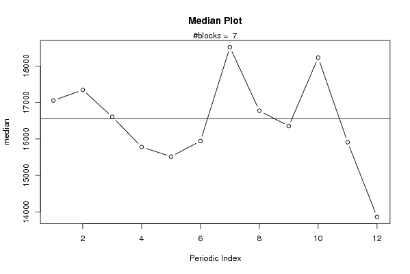
| Title produced by software | Mean Plot | ||||||||||||||||||||
| Date of computation | Sun, 21 Dec 2008 12:58:57 -0700 | ||||||||||||||||||||
| Cite this page as follows | Statistical Computations at FreeStatistics.org, Office for Research Development and Education, URL https://freestatistics.org/blog/index.php?v=date/2008/Dec/21/t12298895622dbrwkx23b97sfp.htm/, Retrieved Sun, 19 May 2024 09:20:16 +0000 | ||||||||||||||||||||
| Statistical Computations at FreeStatistics.org, Office for Research Development and Education, URL https://freestatistics.org/blog/index.php?pk=35796, Retrieved Sun, 19 May 2024 09:20:16 +0000 | |||||||||||||||||||||
| QR Codes: | |||||||||||||||||||||
|
| |||||||||||||||||||||
| Original text written by user: | |||||||||||||||||||||
| IsPrivate? | No (this computation is public) | ||||||||||||||||||||
| User-defined keywords | |||||||||||||||||||||
| Estimated Impact | 164 | ||||||||||||||||||||
Tree of Dependent Computations | |||||||||||||||||||||
| Family? (F = Feedback message, R = changed R code, M = changed R Module, P = changed Parameters, D = changed Data) | |||||||||||||||||||||
| F [Univariate Explorative Data Analysis] [Investigating dis...] [2007-10-22 19:45:25] [b9964c45117f7aac638ab9056d451faa] - PD [Univariate Explorative Data Analysis] [Task 3: Buitenlan...] [2008-10-27 19:53:20] [504b73e6de93b01331326637b3288ad4] - PD [Univariate Explorative Data Analysis] [Handelsbalans Belgi�] [2008-12-21 19:07:51] [504b73e6de93b01331326637b3288ad4] - RMPD [Mean Plot] [Mean plot Uitvoer] [2008-12-21 19:58:57] [ba85d9d0a82357dd3edf208eef933423] [Current] | |||||||||||||||||||||
| Feedback Forum | |||||||||||||||||||||
Post a new message | |||||||||||||||||||||
Dataset | |||||||||||||||||||||
| Dataseries X: | |||||||||||||||||||||
15916.4 16535.9 15796 14418.6 15044.5 14944.2 16754.8 14254 15454.9 15644.8 14568.3 12520.2 14803 15873.2 14755.3 12875.1 14291.1 14205.3 15859.4 15258.9 15498.6 15106.5 15023.6 12083 15761.3 16943 15070.3 13659.6 14768.9 14725.1 15998.1 15370.6 14956.9 15469.7 15101.8 11703.7 16283.6 16726.5 14968.9 14861 14583.3 15305.8 17903.9 16379.4 15420.3 17870.5 15912.8 13866.5 17823.2 17872 17420.4 16704.4 15991.2 16583.6 19123.5 17838.7 17209.4 18586.5 16258.1 15141.6 19202.1 17746.5 19090.1 18040.3 17515.5 17751.8 21072.4 17170 19439.5 19795.4 17574.9 16165.4 19464.6 19932.1 19961.2 17343.4 18924.2 18574.1 21350.6 18594.6 19823.1 20844.4 19640.2 17735.4 19813.6 22238.5 20682.2 17818.6 21872.1 22117 21865.9 23451.3 20953.7 22497.3 | |||||||||||||||||||||
Tables (Output of Computation) | |||||||||||||||||||||
| |||||||||||||||||||||
Figures (Output of Computation) | |||||||||||||||||||||
Input Parameters & R Code | |||||||||||||||||||||
| Parameters (Session): | |||||||||||||||||||||
| par1 = 12 ; | |||||||||||||||||||||
| Parameters (R input): | |||||||||||||||||||||
| par1 = 12 ; | |||||||||||||||||||||
| R code (references can be found in the software module): | |||||||||||||||||||||
par1 <- as.numeric(par1) | |||||||||||||||||||||