Free Statistics
of Irreproducible Research!
Description of Statistical Computation | |||||||||||||||||||||||||||||||||||||||||||||||||||||
|---|---|---|---|---|---|---|---|---|---|---|---|---|---|---|---|---|---|---|---|---|---|---|---|---|---|---|---|---|---|---|---|---|---|---|---|---|---|---|---|---|---|---|---|---|---|---|---|---|---|---|---|---|---|
| Author's title | |||||||||||||||||||||||||||||||||||||||||||||||||||||
| Author | *The author of this computation has been verified* | ||||||||||||||||||||||||||||||||||||||||||||||||||||
| R Software Module | rwasp_edauni.wasp | ||||||||||||||||||||||||||||||||||||||||||||||||||||
| Title produced by software | Univariate Explorative Data Analysis | ||||||||||||||||||||||||||||||||||||||||||||||||||||
| Date of computation | Sun, 21 Dec 2008 12:45:59 -0700 | ||||||||||||||||||||||||||||||||||||||||||||||||||||
| Cite this page as follows | Statistical Computations at FreeStatistics.org, Office for Research Development and Education, URL https://freestatistics.org/blog/index.php?v=date/2008/Dec/21/t1229888791lh2bj9bb86hmf96.htm/, Retrieved Sun, 19 May 2024 11:30:45 +0000 | ||||||||||||||||||||||||||||||||||||||||||||||||||||
| Statistical Computations at FreeStatistics.org, Office for Research Development and Education, URL https://freestatistics.org/blog/index.php?pk=35785, Retrieved Sun, 19 May 2024 11:30:45 +0000 | |||||||||||||||||||||||||||||||||||||||||||||||||||||
| QR Codes: | |||||||||||||||||||||||||||||||||||||||||||||||||||||
|
| |||||||||||||||||||||||||||||||||||||||||||||||||||||
| Original text written by user: | |||||||||||||||||||||||||||||||||||||||||||||||||||||
| IsPrivate? | No (this computation is public) | ||||||||||||||||||||||||||||||||||||||||||||||||||||
| User-defined keywords | |||||||||||||||||||||||||||||||||||||||||||||||||||||
| Estimated Impact | 140 | ||||||||||||||||||||||||||||||||||||||||||||||||||||
Tree of Dependent Computations | |||||||||||||||||||||||||||||||||||||||||||||||||||||
| Family? (F = Feedback message, R = changed R code, M = changed R Module, P = changed Parameters, D = changed Data) | |||||||||||||||||||||||||||||||||||||||||||||||||||||
| F [Univariate Explorative Data Analysis] [Investigating dis...] [2007-10-22 19:45:25] [b9964c45117f7aac638ab9056d451faa] - PD [Univariate Explorative Data Analysis] [Task 3: Buitenlan...] [2008-10-27 19:53:20] [504b73e6de93b01331326637b3288ad4] - PD [Univariate Explorative Data Analysis] [Handelsbalans Belgi�] [2008-12-21 19:07:51] [504b73e6de93b01331326637b3288ad4] - D [Univariate Explorative Data Analysis] [Handelsbalans Belgi�] [2008-12-21 19:45:59] [ba85d9d0a82357dd3edf208eef933423] [Current] | |||||||||||||||||||||||||||||||||||||||||||||||||||||
| Feedback Forum | |||||||||||||||||||||||||||||||||||||||||||||||||||||
Post a new message | |||||||||||||||||||||||||||||||||||||||||||||||||||||
Dataset | |||||||||||||||||||||||||||||||||||||||||||||||||||||
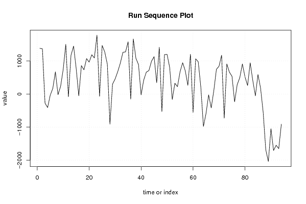
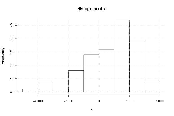
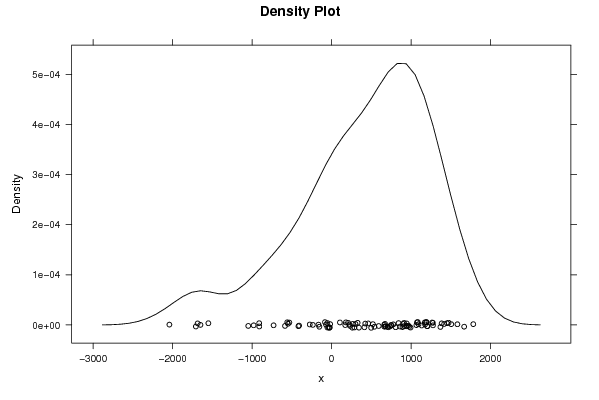
| Dataseries X: | |||||||||||||||||||||||||||||||||||||||||||||||||||||
1384,2 1368,9 -275,1 -408,9 -37,5 171,5 671,8 -18,5 231,6 747,5 1505,7 -83,6 1173,2 1452,1 777 -52,8 861,2 735,2 1073,6 966,9 1189,8 1093,5 1782,7 -70,4 1471,6 1273,8 900,8 -910,2 299,8 460,2 677,2 937,1 1265,4 1275,6 1582,6 -154,2 1667,6 1083,1 891,7 -26,5 423,4 662,8 711,4 993,3 1133,2 343,9 1415,8 -531,8 1193,6 1201,3 805,6 -164,8 327,3 223,7 675,8 949,7 704,4 265,6 1206 -558,2 1066,8 977,8 207,1 -980,7 -586,4 -24,3 -417,5 104,7 749,5 842,3 1176 -730,3 911,6 662,1 539,1 -236 286,9 497,4 912 519,4 260,1 945,2 412,7 -54,2 592,8 179,9 -548,6 -1685,8 -2041 -1048,7 -1708,4 -1550,7 -1650,2 -911,3 | |||||||||||||||||||||||||||||||||||||||||||||||||||||
Tables (Output of Computation) | |||||||||||||||||||||||||||||||||||||||||||||||||||||
| |||||||||||||||||||||||||||||||||||||||||||||||||||||
Figures (Output of Computation) | |||||||||||||||||||||||||||||||||||||||||||||||||||||
Input Parameters & R Code | |||||||||||||||||||||||||||||||||||||||||||||||||||||
| Parameters (Session): | |||||||||||||||||||||||||||||||||||||||||||||||||||||
| par1 = 0 ; par2 = 0 ; | |||||||||||||||||||||||||||||||||||||||||||||||||||||
| Parameters (R input): | |||||||||||||||||||||||||||||||||||||||||||||||||||||
| par1 = 0 ; par2 = 0 ; | |||||||||||||||||||||||||||||||||||||||||||||||||||||
| R code (references can be found in the software module): | |||||||||||||||||||||||||||||||||||||||||||||||||||||
par1 <- as.numeric(par1) | |||||||||||||||||||||||||||||||||||||||||||||||||||||