Repository of Reproducible Computations

Free Statistics

of Irreproducible Research!

Author's title

Author

*Unverified author*

R Software Module

rwasp_autocorrelation.wasp

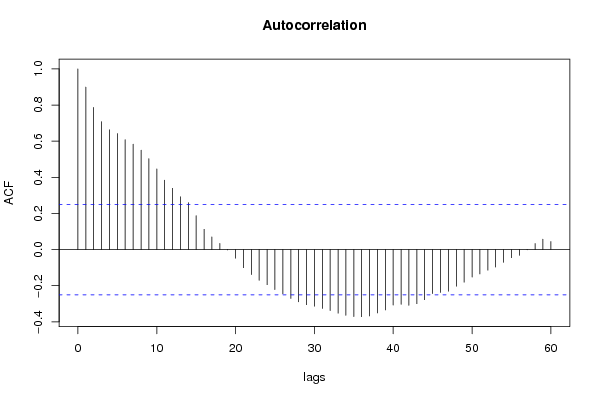
Title produced by software

(Partial) Autocorrelation Function

Date of computation

Sat, 20 Dec 2008 07:46:30 -0700

Cite this page as follows

Statistical Computations at FreeStatistics.org, Office for Research Development and Education, URL https://freestatistics.org/blog/index.php?v=date/2008/Dec/20/t1229784484qei9fn91wn55duy.htm/, Retrieved Sun, 19 May 2024 09:36:58 +0000

Statistical Computations at FreeStatistics.org, Office for Research Development and Education, URL https://freestatistics.org/blog/index.php?pk=35390, Retrieved Sun, 19 May 2024 09:36:58 +0000

QR Codes:

Paste this QR Code to cite your computation.

Original text written by user:

IsPrivate?

No (this computation is public)

User-defined keywords

Estimated Impact

198

Family? (F = Feedback message, R = changed R code, M = changed R Module, P = changed Parameters, D = changed Data)

F     [(Partial) Autocorrelation Function] [Step 2 ACF zonder...] [2008-12-10 00:24:04] [7a4703cb85a198d9845d72899eff0288]
-    D    [(Partial) Autocorrelation Function] [PaperACF1Geoffrey] [2008-12-20 14:46:30] [9bd6ffcbd02a1b442f4187c5798ef35f] [Current]

Feedback Forum

Post a new message

Dataseries X:

Download CSV

Histogram

Boxplots

Summary of computational transaction
Raw Input	view raw input (R code)
Raw Output	view raw output of R engine
Computing time	2 seconds
R Server	'Gwilym Jenkins' @ 72.249.127.135

\begin{tabular}{lllllllll}
\hline
Summary of computational transaction \tabularnewline
Raw Input & view raw input (R code)  \tabularnewline
Raw Output & view raw output of R engine  \tabularnewline
Computing time & 2 seconds \tabularnewline
R Server & 'Gwilym Jenkins' @ 72.249.127.135 \tabularnewline
\hline
\end{tabular}
%Source: https://freestatistics.org/blog/index.php?pk=35390&T=0

[TABLE]
[ROW][C]Summary of computational transaction[/C][/ROW]
[ROW][C]Raw Input[/C][C]view raw input (R code) [/C][/ROW]
[ROW][C]Raw Output[/C][C]view raw output of R engine [/C][/ROW]
[ROW][C]Computing time[/C][C]2 seconds[/C][/ROW]
[ROW][C]R Server[/C][C]'Gwilym Jenkins' @ 72.249.127.135[/C][/ROW]
[/TABLE]
Source: https://freestatistics.org/blog/index.php?pk=35390&T=0

Globally Unique Identifier (entire table): ba.freestatistics.org/blog/index.php?pk=35390&T=0

As an alternative you can also use a QR Code:

The GUIDs for individual cells are displayed in the table below:

Summary of computational transaction
Raw Input	view raw input (R code)
Raw Output	view raw output of R engine
Computing time	2 seconds
R Server	'Gwilym Jenkins' @ 72.249.127.135

Autocorrelation Function
Time lag k	ACF(k)	T-STAT	P-value
1	0.899428	7.0248	0
2	0.786733	6.1446	0
3	0.708086	5.5303	0
4	0.663377	5.1811	1e-06
5	0.642665	5.0194	2e-06
6	0.608494	4.7525	6e-06
7	0.583228	4.5552	1.3e-05
8	0.549969	4.2954	3.2e-05
9	0.503015	3.9287	0.00011
10	0.446609	3.4881	0.000454
11	0.38396	2.9988	0.001959
12	0.338961	2.6474	0.005155
13	0.292212	2.2823	0.012988
14	0.25939	2.0259	0.023577
15	0.18795	1.4679	0.073629
16	0.11253	0.8789	0.191456
17	0.070018	0.5469	0.293235
18	0.034344	0.2682	0.394712
19	-0.00163	-0.0127	0.494941
20	-0.047504	-0.371	0.355955
21	-0.100341	-0.7837	0.218127
22	-0.138541	-1.082	0.141747
23	-0.170156	-1.329	0.094405
24	-0.194625	-1.5201	0.06683
25	-0.221552	-1.7304	0.044309
26	-0.244582	-1.9102	0.030403
27	-0.270283	-2.111	0.01944
28	-0.288972	-2.2569	0.013802
29	-0.304922	-2.3815	0.010189
30	-0.313261	-2.4466	0.008658
31	-0.326135	-2.5472	0.006698
32	-0.337891	-2.639	0.00527
33	-0.351995	-2.7492	0.003925
34	-0.363733	-2.8408	0.003054
35	-0.370785	-2.8959	0.00262
36	-0.371287	-2.8998	0.002592
37	-0.367548	-2.8706	0.002812
38	-0.350697	-2.739	0.004034
39	-0.334026	-2.6088	0.005705
40	-0.306847	-2.3966	0.009815
41	-0.302752	-2.3646	0.010624
42	-0.308512	-2.4096	0.009502
43	-0.299782	-2.3414	0.011248
44	-0.277568	-2.1679	0.01704
45	-0.243729	-1.9036	0.030843
46	-0.237523	-1.8551	0.034207
47	-0.230575	-1.8008	0.038335
48	-0.20263	-1.5826	0.059343
49	-0.180257	-1.4079	0.082125
50	-0.152267	-1.1892	0.119476
51	-0.135078	-1.055	0.147794
52	-0.11376	-0.8885	0.188883
53	-0.096875	-0.7566	0.226096
54	-0.070245	-0.5486	0.29263
55	-0.044671	-0.3489	0.364185
56	-0.032007	-0.25	0.40172
57	-0.001296	-0.0101	0.495977
58	0.03348	0.2615	0.397298
59	0.057835	0.4517	0.326541
60	0.044559	0.348	0.364514

\begin{tabular}{lllllllll}
\hline
Autocorrelation Function \tabularnewline
Time lag k & ACF(k) & T-STAT & P-value \tabularnewline
1 & 0.899428 & 7.0248 & 0 \tabularnewline
2 & 0.786733 & 6.1446 & 0 \tabularnewline
3 & 0.708086 & 5.5303 & 0 \tabularnewline
4 & 0.663377 & 5.1811 & 1e-06 \tabularnewline
5 & 0.642665 & 5.0194 & 2e-06 \tabularnewline
6 & 0.608494 & 4.7525 & 6e-06 \tabularnewline
7 & 0.583228 & 4.5552 & 1.3e-05 \tabularnewline
8 & 0.549969 & 4.2954 & 3.2e-05 \tabularnewline
9 & 0.503015 & 3.9287 & 0.00011 \tabularnewline
10 & 0.446609 & 3.4881 & 0.000454 \tabularnewline
11 & 0.38396 & 2.9988 & 0.001959 \tabularnewline
12 & 0.338961 & 2.6474 & 0.005155 \tabularnewline
13 & 0.292212 & 2.2823 & 0.012988 \tabularnewline
14 & 0.25939 & 2.0259 & 0.023577 \tabularnewline
15 & 0.18795 & 1.4679 & 0.073629 \tabularnewline
16 & 0.11253 & 0.8789 & 0.191456 \tabularnewline
17 & 0.070018 & 0.5469 & 0.293235 \tabularnewline
18 & 0.034344 & 0.2682 & 0.394712 \tabularnewline
19 & -0.00163 & -0.0127 & 0.494941 \tabularnewline
20 & -0.047504 & -0.371 & 0.355955 \tabularnewline
21 & -0.100341 & -0.7837 & 0.218127 \tabularnewline
22 & -0.138541 & -1.082 & 0.141747 \tabularnewline
23 & -0.170156 & -1.329 & 0.094405 \tabularnewline
24 & -0.194625 & -1.5201 & 0.06683 \tabularnewline
25 & -0.221552 & -1.7304 & 0.044309 \tabularnewline
26 & -0.244582 & -1.9102 & 0.030403 \tabularnewline
27 & -0.270283 & -2.111 & 0.01944 \tabularnewline
28 & -0.288972 & -2.2569 & 0.013802 \tabularnewline
29 & -0.304922 & -2.3815 & 0.010189 \tabularnewline
30 & -0.313261 & -2.4466 & 0.008658 \tabularnewline
31 & -0.326135 & -2.5472 & 0.006698 \tabularnewline
32 & -0.337891 & -2.639 & 0.00527 \tabularnewline
33 & -0.351995 & -2.7492 & 0.003925 \tabularnewline
34 & -0.363733 & -2.8408 & 0.003054 \tabularnewline
35 & -0.370785 & -2.8959 & 0.00262 \tabularnewline
36 & -0.371287 & -2.8998 & 0.002592 \tabularnewline
37 & -0.367548 & -2.8706 & 0.002812 \tabularnewline
38 & -0.350697 & -2.739 & 0.004034 \tabularnewline
39 & -0.334026 & -2.6088 & 0.005705 \tabularnewline
40 & -0.306847 & -2.3966 & 0.009815 \tabularnewline
41 & -0.302752 & -2.3646 & 0.010624 \tabularnewline
42 & -0.308512 & -2.4096 & 0.009502 \tabularnewline
43 & -0.299782 & -2.3414 & 0.011248 \tabularnewline
44 & -0.277568 & -2.1679 & 0.01704 \tabularnewline
45 & -0.243729 & -1.9036 & 0.030843 \tabularnewline
46 & -0.237523 & -1.8551 & 0.034207 \tabularnewline
47 & -0.230575 & -1.8008 & 0.038335 \tabularnewline
48 & -0.20263 & -1.5826 & 0.059343 \tabularnewline
49 & -0.180257 & -1.4079 & 0.082125 \tabularnewline
50 & -0.152267 & -1.1892 & 0.119476 \tabularnewline
51 & -0.135078 & -1.055 & 0.147794 \tabularnewline
52 & -0.11376 & -0.8885 & 0.188883 \tabularnewline
53 & -0.096875 & -0.7566 & 0.226096 \tabularnewline
54 & -0.070245 & -0.5486 & 0.29263 \tabularnewline
55 & -0.044671 & -0.3489 & 0.364185 \tabularnewline
56 & -0.032007 & -0.25 & 0.40172 \tabularnewline
57 & -0.001296 & -0.0101 & 0.495977 \tabularnewline
58 & 0.03348 & 0.2615 & 0.397298 \tabularnewline
59 & 0.057835 & 0.4517 & 0.326541 \tabularnewline
60 & 0.044559 & 0.348 & 0.364514 \tabularnewline
\hline
\end{tabular}
%Source: https://freestatistics.org/blog/index.php?pk=35390&T=1

[TABLE]
[ROW][C]Autocorrelation Function[/C][/ROW]
[ROW][C]Time lag k[/C][C]ACF(k)[/C][C]T-STAT[/C][C]P-value[/C][/ROW]
[ROW][C]1[/C][C]0.899428[/C][C]7.0248[/C][C]0[/C][/ROW]
[ROW][C]2[/C][C]0.786733[/C][C]6.1446[/C][C]0[/C][/ROW]
[ROW][C]3[/C][C]0.708086[/C][C]5.5303[/C][C]0[/C][/ROW]
[ROW][C]4[/C][C]0.663377[/C][C]5.1811[/C][C]1e-06[/C][/ROW]
[ROW][C]5[/C][C]0.642665[/C][C]5.0194[/C][C]2e-06[/C][/ROW]
[ROW][C]6[/C][C]0.608494[/C][C]4.7525[/C][C]6e-06[/C][/ROW]
[ROW][C]7[/C][C]0.583228[/C][C]4.5552[/C][C]1.3e-05[/C][/ROW]
[ROW][C]8[/C][C]0.549969[/C][C]4.2954[/C][C]3.2e-05[/C][/ROW]
[ROW][C]9[/C][C]0.503015[/C][C]3.9287[/C][C]0.00011[/C][/ROW]
[ROW][C]10[/C][C]0.446609[/C][C]3.4881[/C][C]0.000454[/C][/ROW]
[ROW][C]11[/C][C]0.38396[/C][C]2.9988[/C][C]0.001959[/C][/ROW]
[ROW][C]12[/C][C]0.338961[/C][C]2.6474[/C][C]0.005155[/C][/ROW]
[ROW][C]13[/C][C]0.292212[/C][C]2.2823[/C][C]0.012988[/C][/ROW]
[ROW][C]14[/C][C]0.25939[/C][C]2.0259[/C][C]0.023577[/C][/ROW]
[ROW][C]15[/C][C]0.18795[/C][C]1.4679[/C][C]0.073629[/C][/ROW]
[ROW][C]16[/C][C]0.11253[/C][C]0.8789[/C][C]0.191456[/C][/ROW]
[ROW][C]17[/C][C]0.070018[/C][C]0.5469[/C][C]0.293235[/C][/ROW]
[ROW][C]18[/C][C]0.034344[/C][C]0.2682[/C][C]0.394712[/C][/ROW]
[ROW][C]19[/C][C]-0.00163[/C][C]-0.0127[/C][C]0.494941[/C][/ROW]
[ROW][C]20[/C][C]-0.047504[/C][C]-0.371[/C][C]0.355955[/C][/ROW]
[ROW][C]21[/C][C]-0.100341[/C][C]-0.7837[/C][C]0.218127[/C][/ROW]
[ROW][C]22[/C][C]-0.138541[/C][C]-1.082[/C][C]0.141747[/C][/ROW]
[ROW][C]23[/C][C]-0.170156[/C][C]-1.329[/C][C]0.094405[/C][/ROW]
[ROW][C]24[/C][C]-0.194625[/C][C]-1.5201[/C][C]0.06683[/C][/ROW]
[ROW][C]25[/C][C]-0.221552[/C][C]-1.7304[/C][C]0.044309[/C][/ROW]
[ROW][C]26[/C][C]-0.244582[/C][C]-1.9102[/C][C]0.030403[/C][/ROW]
[ROW][C]27[/C][C]-0.270283[/C][C]-2.111[/C][C]0.01944[/C][/ROW]
[ROW][C]28[/C][C]-0.288972[/C][C]-2.2569[/C][C]0.013802[/C][/ROW]
[ROW][C]29[/C][C]-0.304922[/C][C]-2.3815[/C][C]0.010189[/C][/ROW]
[ROW][C]30[/C][C]-0.313261[/C][C]-2.4466[/C][C]0.008658[/C][/ROW]
[ROW][C]31[/C][C]-0.326135[/C][C]-2.5472[/C][C]0.006698[/C][/ROW]
[ROW][C]32[/C][C]-0.337891[/C][C]-2.639[/C][C]0.00527[/C][/ROW]
[ROW][C]33[/C][C]-0.351995[/C][C]-2.7492[/C][C]0.003925[/C][/ROW]
[ROW][C]34[/C][C]-0.363733[/C][C]-2.8408[/C][C]0.003054[/C][/ROW]
[ROW][C]35[/C][C]-0.370785[/C][C]-2.8959[/C][C]0.00262[/C][/ROW]
[ROW][C]36[/C][C]-0.371287[/C][C]-2.8998[/C][C]0.002592[/C][/ROW]
[ROW][C]37[/C][C]-0.367548[/C][C]-2.8706[/C][C]0.002812[/C][/ROW]
[ROW][C]38[/C][C]-0.350697[/C][C]-2.739[/C][C]0.004034[/C][/ROW]
[ROW][C]39[/C][C]-0.334026[/C][C]-2.6088[/C][C]0.005705[/C][/ROW]
[ROW][C]40[/C][C]-0.306847[/C][C]-2.3966[/C][C]0.009815[/C][/ROW]
[ROW][C]41[/C][C]-0.302752[/C][C]-2.3646[/C][C]0.010624[/C][/ROW]
[ROW][C]42[/C][C]-0.308512[/C][C]-2.4096[/C][C]0.009502[/C][/ROW]
[ROW][C]43[/C][C]-0.299782[/C][C]-2.3414[/C][C]0.011248[/C][/ROW]
[ROW][C]44[/C][C]-0.277568[/C][C]-2.1679[/C][C]0.01704[/C][/ROW]
[ROW][C]45[/C][C]-0.243729[/C][C]-1.9036[/C][C]0.030843[/C][/ROW]
[ROW][C]46[/C][C]-0.237523[/C][C]-1.8551[/C][C]0.034207[/C][/ROW]
[ROW][C]47[/C][C]-0.230575[/C][C]-1.8008[/C][C]0.038335[/C][/ROW]
[ROW][C]48[/C][C]-0.20263[/C][C]-1.5826[/C][C]0.059343[/C][/ROW]
[ROW][C]49[/C][C]-0.180257[/C][C]-1.4079[/C][C]0.082125[/C][/ROW]
[ROW][C]50[/C][C]-0.152267[/C][C]-1.1892[/C][C]0.119476[/C][/ROW]
[ROW][C]51[/C][C]-0.135078[/C][C]-1.055[/C][C]0.147794[/C][/ROW]
[ROW][C]52[/C][C]-0.11376[/C][C]-0.8885[/C][C]0.188883[/C][/ROW]
[ROW][C]53[/C][C]-0.096875[/C][C]-0.7566[/C][C]0.226096[/C][/ROW]
[ROW][C]54[/C][C]-0.070245[/C][C]-0.5486[/C][C]0.29263[/C][/ROW]
[ROW][C]55[/C][C]-0.044671[/C][C]-0.3489[/C][C]0.364185[/C][/ROW]
[ROW][C]56[/C][C]-0.032007[/C][C]-0.25[/C][C]0.40172[/C][/ROW]
[ROW][C]57[/C][C]-0.001296[/C][C]-0.0101[/C][C]0.495977[/C][/ROW]
[ROW][C]58[/C][C]0.03348[/C][C]0.2615[/C][C]0.397298[/C][/ROW]
[ROW][C]59[/C][C]0.057835[/C][C]0.4517[/C][C]0.326541[/C][/ROW]
[ROW][C]60[/C][C]0.044559[/C][C]0.348[/C][C]0.364514[/C][/ROW]
[/TABLE]
Source: https://freestatistics.org/blog/index.php?pk=35390&T=1

Globally Unique Identifier (entire table): ba.freestatistics.org/blog/index.php?pk=35390&T=1

As an alternative you can also use a QR Code:

The GUIDs for individual cells are displayed in the table below:

Autocorrelation Function
Time lag k	ACF(k)	T-STAT	P-value
1	0.899428	7.0248	0
2	0.786733	6.1446	0
3	0.708086	5.5303	0
4	0.663377	5.1811	1e-06
5	0.642665	5.0194	2e-06
6	0.608494	4.7525	6e-06
7	0.583228	4.5552	1.3e-05
8	0.549969	4.2954	3.2e-05
9	0.503015	3.9287	0.00011
10	0.446609	3.4881	0.000454
11	0.38396	2.9988	0.001959
12	0.338961	2.6474	0.005155
13	0.292212	2.2823	0.012988
14	0.25939	2.0259	0.023577
15	0.18795	1.4679	0.073629
16	0.11253	0.8789	0.191456
17	0.070018	0.5469	0.293235
18	0.034344	0.2682	0.394712
19	-0.00163	-0.0127	0.494941
20	-0.047504	-0.371	0.355955
21	-0.100341	-0.7837	0.218127
22	-0.138541	-1.082	0.141747
23	-0.170156	-1.329	0.094405
24	-0.194625	-1.5201	0.06683
25	-0.221552	-1.7304	0.044309
26	-0.244582	-1.9102	0.030403
27	-0.270283	-2.111	0.01944
28	-0.288972	-2.2569	0.013802
29	-0.304922	-2.3815	0.010189
30	-0.313261	-2.4466	0.008658
31	-0.326135	-2.5472	0.006698
32	-0.337891	-2.639	0.00527
33	-0.351995	-2.7492	0.003925
34	-0.363733	-2.8408	0.003054
35	-0.370785	-2.8959	0.00262
36	-0.371287	-2.8998	0.002592
37	-0.367548	-2.8706	0.002812
38	-0.350697	-2.739	0.004034
39	-0.334026	-2.6088	0.005705
40	-0.306847	-2.3966	0.009815
41	-0.302752	-2.3646	0.010624
42	-0.308512	-2.4096	0.009502
43	-0.299782	-2.3414	0.011248
44	-0.277568	-2.1679	0.01704
45	-0.243729	-1.9036	0.030843
46	-0.237523	-1.8551	0.034207
47	-0.230575	-1.8008	0.038335
48	-0.20263	-1.5826	0.059343
49	-0.180257	-1.4079	0.082125
50	-0.152267	-1.1892	0.119476
51	-0.135078	-1.055	0.147794
52	-0.11376	-0.8885	0.188883
53	-0.096875	-0.7566	0.226096
54	-0.070245	-0.5486	0.29263
55	-0.044671	-0.3489	0.364185
56	-0.032007	-0.25	0.40172
57	-0.001296	-0.0101	0.495977
58	0.03348	0.2615	0.397298
59	0.057835	0.4517	0.326541
60	0.044559	0.348	0.364514

Partial Autocorrelation Function
Time lag k	PACF(k)	T-STAT	P-value
1	0.899428	7.0248	0
2	-0.116414	-0.9092	0.183405
3	0.121031	0.9453	0.174121
4	0.111627	0.8718	0.193359
5	0.107117	0.8366	0.203039
6	-0.052473	-0.4098	0.341684
7	0.099447	0.7767	0.220166
8	-0.046927	-0.3665	0.357625
9	-0.061806	-0.4827	0.31551
10	-0.07542	-0.589	0.279002
11	-0.070536	-0.5509	0.291857
12	0.007139	0.0558	0.477858
13	-0.086314	-0.6741	0.251387
14	0.043949	0.3433	0.366295
15	-0.265052	-2.0701	0.021341
16	-0.01284	-0.1003	0.460223
17	0.05619	0.4389	0.331158
18	-0.04036	-0.3152	0.376833
19	-0.0647	-0.5053	0.307577
20	-0.014033	-0.1096	0.456542
21	-0.083036	-0.6485	0.259539
22	0.017739	0.1385	0.445131
23	0.016025	0.1252	0.450405
24	0.000247	0.0019	0.499233
25	-0.022187	-0.1733	0.431499
26	-0.015048	-0.1175	0.453414
27	-0.031099	-0.2429	0.404452
28	0.003791	0.0296	0.488239
29	0.015233	0.119	0.452845
30	0.043571	0.3403	0.367399
31	-0.119932	-0.9367	0.176303
32	-0.00369	-0.0288	0.488552
33	-0.031721	-0.2477	0.402581
34	-0.026187	-0.2045	0.41931
35	-0.006453	-0.0504	0.479985
36	-0.014421	-0.1126	0.455346
37	-0.043402	-0.339	0.367894
38	0.058083	0.4536	0.325849
39	0.007498	0.0586	0.476748
40	0.078032	0.6094	0.272245
41	-0.114751	-0.8962	0.186825
42	-0.037217	-0.2907	0.386144
43	0.046355	0.362	0.359284
44	0.003863	0.0302	0.488014
45	0.065565	0.5121	0.305223
46	-0.147511	-1.1521	0.126887
47	0.024785	0.1936	0.423575
48	0.061176	0.4778	0.31725
49	-0.046401	-0.3624	0.359151
50	0.031863	0.2489	0.402153
51	0.008349	0.0652	0.474112
52	-0.041807	-0.3265	0.372572
53	-0.032241	-0.2518	0.401016
54	0.069803	0.5452	0.293809
55	-0.002205	-0.0172	0.493157
56	-0.005054	-0.0395	0.48432
57	0.055432	0.4329	0.333293
58	0.012492	0.0976	0.461299
59	-0.070042	-0.547	0.293171
60	-0.133442	-1.0422	0.150713

\begin{tabular}{lllllllll}
\hline
Partial Autocorrelation Function \tabularnewline
Time lag k & PACF(k) & T-STAT & P-value \tabularnewline
1 & 0.899428 & 7.0248 & 0 \tabularnewline
2 & -0.116414 & -0.9092 & 0.183405 \tabularnewline
3 & 0.121031 & 0.9453 & 0.174121 \tabularnewline
4 & 0.111627 & 0.8718 & 0.193359 \tabularnewline
5 & 0.107117 & 0.8366 & 0.203039 \tabularnewline
6 & -0.052473 & -0.4098 & 0.341684 \tabularnewline
7 & 0.099447 & 0.7767 & 0.220166 \tabularnewline
8 & -0.046927 & -0.3665 & 0.357625 \tabularnewline
9 & -0.061806 & -0.4827 & 0.31551 \tabularnewline
10 & -0.07542 & -0.589 & 0.279002 \tabularnewline
11 & -0.070536 & -0.5509 & 0.291857 \tabularnewline
12 & 0.007139 & 0.0558 & 0.477858 \tabularnewline
13 & -0.086314 & -0.6741 & 0.251387 \tabularnewline
14 & 0.043949 & 0.3433 & 0.366295 \tabularnewline
15 & -0.265052 & -2.0701 & 0.021341 \tabularnewline
16 & -0.01284 & -0.1003 & 0.460223 \tabularnewline
17 & 0.05619 & 0.4389 & 0.331158 \tabularnewline
18 & -0.04036 & -0.3152 & 0.376833 \tabularnewline
19 & -0.0647 & -0.5053 & 0.307577 \tabularnewline
20 & -0.014033 & -0.1096 & 0.456542 \tabularnewline
21 & -0.083036 & -0.6485 & 0.259539 \tabularnewline
22 & 0.017739 & 0.1385 & 0.445131 \tabularnewline
23 & 0.016025 & 0.1252 & 0.450405 \tabularnewline
24 & 0.000247 & 0.0019 & 0.499233 \tabularnewline
25 & -0.022187 & -0.1733 & 0.431499 \tabularnewline
26 & -0.015048 & -0.1175 & 0.453414 \tabularnewline
27 & -0.031099 & -0.2429 & 0.404452 \tabularnewline
28 & 0.003791 & 0.0296 & 0.488239 \tabularnewline
29 & 0.015233 & 0.119 & 0.452845 \tabularnewline
30 & 0.043571 & 0.3403 & 0.367399 \tabularnewline
31 & -0.119932 & -0.9367 & 0.176303 \tabularnewline
32 & -0.00369 & -0.0288 & 0.488552 \tabularnewline
33 & -0.031721 & -0.2477 & 0.402581 \tabularnewline
34 & -0.026187 & -0.2045 & 0.41931 \tabularnewline
35 & -0.006453 & -0.0504 & 0.479985 \tabularnewline
36 & -0.014421 & -0.1126 & 0.455346 \tabularnewline
37 & -0.043402 & -0.339 & 0.367894 \tabularnewline
38 & 0.058083 & 0.4536 & 0.325849 \tabularnewline
39 & 0.007498 & 0.0586 & 0.476748 \tabularnewline
40 & 0.078032 & 0.6094 & 0.272245 \tabularnewline
41 & -0.114751 & -0.8962 & 0.186825 \tabularnewline
42 & -0.037217 & -0.2907 & 0.386144 \tabularnewline
43 & 0.046355 & 0.362 & 0.359284 \tabularnewline
44 & 0.003863 & 0.0302 & 0.488014 \tabularnewline
45 & 0.065565 & 0.5121 & 0.305223 \tabularnewline
46 & -0.147511 & -1.1521 & 0.126887 \tabularnewline
47 & 0.024785 & 0.1936 & 0.423575 \tabularnewline
48 & 0.061176 & 0.4778 & 0.31725 \tabularnewline
49 & -0.046401 & -0.3624 & 0.359151 \tabularnewline
50 & 0.031863 & 0.2489 & 0.402153 \tabularnewline
51 & 0.008349 & 0.0652 & 0.474112 \tabularnewline
52 & -0.041807 & -0.3265 & 0.372572 \tabularnewline
53 & -0.032241 & -0.2518 & 0.401016 \tabularnewline
54 & 0.069803 & 0.5452 & 0.293809 \tabularnewline
55 & -0.002205 & -0.0172 & 0.493157 \tabularnewline
56 & -0.005054 & -0.0395 & 0.48432 \tabularnewline
57 & 0.055432 & 0.4329 & 0.333293 \tabularnewline
58 & 0.012492 & 0.0976 & 0.461299 \tabularnewline
59 & -0.070042 & -0.547 & 0.293171 \tabularnewline
60 & -0.133442 & -1.0422 & 0.150713 \tabularnewline
\hline
\end{tabular}
%Source: https://freestatistics.org/blog/index.php?pk=35390&T=2

[TABLE]
[ROW][C]Partial Autocorrelation Function[/C][/ROW]
[ROW][C]Time lag k[/C][C]PACF(k)[/C][C]T-STAT[/C][C]P-value[/C][/ROW]
[ROW][C]1[/C][C]0.899428[/C][C]7.0248[/C][C]0[/C][/ROW]
[ROW][C]2[/C][C]-0.116414[/C][C]-0.9092[/C][C]0.183405[/C][/ROW]
[ROW][C]3[/C][C]0.121031[/C][C]0.9453[/C][C]0.174121[/C][/ROW]
[ROW][C]4[/C][C]0.111627[/C][C]0.8718[/C][C]0.193359[/C][/ROW]
[ROW][C]5[/C][C]0.107117[/C][C]0.8366[/C][C]0.203039[/C][/ROW]
[ROW][C]6[/C][C]-0.052473[/C][C]-0.4098[/C][C]0.341684[/C][/ROW]
[ROW][C]7[/C][C]0.099447[/C][C]0.7767[/C][C]0.220166[/C][/ROW]
[ROW][C]8[/C][C]-0.046927[/C][C]-0.3665[/C][C]0.357625[/C][/ROW]
[ROW][C]9[/C][C]-0.061806[/C][C]-0.4827[/C][C]0.31551[/C][/ROW]
[ROW][C]10[/C][C]-0.07542[/C][C]-0.589[/C][C]0.279002[/C][/ROW]
[ROW][C]11[/C][C]-0.070536[/C][C]-0.5509[/C][C]0.291857[/C][/ROW]
[ROW][C]12[/C][C]0.007139[/C][C]0.0558[/C][C]0.477858[/C][/ROW]
[ROW][C]13[/C][C]-0.086314[/C][C]-0.6741[/C][C]0.251387[/C][/ROW]
[ROW][C]14[/C][C]0.043949[/C][C]0.3433[/C][C]0.366295[/C][/ROW]
[ROW][C]15[/C][C]-0.265052[/C][C]-2.0701[/C][C]0.021341[/C][/ROW]
[ROW][C]16[/C][C]-0.01284[/C][C]-0.1003[/C][C]0.460223[/C][/ROW]
[ROW][C]17[/C][C]0.05619[/C][C]0.4389[/C][C]0.331158[/C][/ROW]
[ROW][C]18[/C][C]-0.04036[/C][C]-0.3152[/C][C]0.376833[/C][/ROW]
[ROW][C]19[/C][C]-0.0647[/C][C]-0.5053[/C][C]0.307577[/C][/ROW]
[ROW][C]20[/C][C]-0.014033[/C][C]-0.1096[/C][C]0.456542[/C][/ROW]
[ROW][C]21[/C][C]-0.083036[/C][C]-0.6485[/C][C]0.259539[/C][/ROW]
[ROW][C]22[/C][C]0.017739[/C][C]0.1385[/C][C]0.445131[/C][/ROW]
[ROW][C]23[/C][C]0.016025[/C][C]0.1252[/C][C]0.450405[/C][/ROW]
[ROW][C]24[/C][C]0.000247[/C][C]0.0019[/C][C]0.499233[/C][/ROW]
[ROW][C]25[/C][C]-0.022187[/C][C]-0.1733[/C][C]0.431499[/C][/ROW]
[ROW][C]26[/C][C]-0.015048[/C][C]-0.1175[/C][C]0.453414[/C][/ROW]
[ROW][C]27[/C][C]-0.031099[/C][C]-0.2429[/C][C]0.404452[/C][/ROW]
[ROW][C]28[/C][C]0.003791[/C][C]0.0296[/C][C]0.488239[/C][/ROW]
[ROW][C]29[/C][C]0.015233[/C][C]0.119[/C][C]0.452845[/C][/ROW]
[ROW][C]30[/C][C]0.043571[/C][C]0.3403[/C][C]0.367399[/C][/ROW]
[ROW][C]31[/C][C]-0.119932[/C][C]-0.9367[/C][C]0.176303[/C][/ROW]
[ROW][C]32[/C][C]-0.00369[/C][C]-0.0288[/C][C]0.488552[/C][/ROW]
[ROW][C]33[/C][C]-0.031721[/C][C]-0.2477[/C][C]0.402581[/C][/ROW]
[ROW][C]34[/C][C]-0.026187[/C][C]-0.2045[/C][C]0.41931[/C][/ROW]
[ROW][C]35[/C][C]-0.006453[/C][C]-0.0504[/C][C]0.479985[/C][/ROW]
[ROW][C]36[/C][C]-0.014421[/C][C]-0.1126[/C][C]0.455346[/C][/ROW]
[ROW][C]37[/C][C]-0.043402[/C][C]-0.339[/C][C]0.367894[/C][/ROW]
[ROW][C]38[/C][C]0.058083[/C][C]0.4536[/C][C]0.325849[/C][/ROW]
[ROW][C]39[/C][C]0.007498[/C][C]0.0586[/C][C]0.476748[/C][/ROW]
[ROW][C]40[/C][C]0.078032[/C][C]0.6094[/C][C]0.272245[/C][/ROW]
[ROW][C]41[/C][C]-0.114751[/C][C]-0.8962[/C][C]0.186825[/C][/ROW]
[ROW][C]42[/C][C]-0.037217[/C][C]-0.2907[/C][C]0.386144[/C][/ROW]
[ROW][C]43[/C][C]0.046355[/C][C]0.362[/C][C]0.359284[/C][/ROW]
[ROW][C]44[/C][C]0.003863[/C][C]0.0302[/C][C]0.488014[/C][/ROW]
[ROW][C]45[/C][C]0.065565[/C][C]0.5121[/C][C]0.305223[/C][/ROW]
[ROW][C]46[/C][C]-0.147511[/C][C]-1.1521[/C][C]0.126887[/C][/ROW]
[ROW][C]47[/C][C]0.024785[/C][C]0.1936[/C][C]0.423575[/C][/ROW]
[ROW][C]48[/C][C]0.061176[/C][C]0.4778[/C][C]0.31725[/C][/ROW]
[ROW][C]49[/C][C]-0.046401[/C][C]-0.3624[/C][C]0.359151[/C][/ROW]
[ROW][C]50[/C][C]0.031863[/C][C]0.2489[/C][C]0.402153[/C][/ROW]
[ROW][C]51[/C][C]0.008349[/C][C]0.0652[/C][C]0.474112[/C][/ROW]
[ROW][C]52[/C][C]-0.041807[/C][C]-0.3265[/C][C]0.372572[/C][/ROW]
[ROW][C]53[/C][C]-0.032241[/C][C]-0.2518[/C][C]0.401016[/C][/ROW]
[ROW][C]54[/C][C]0.069803[/C][C]0.5452[/C][C]0.293809[/C][/ROW]
[ROW][C]55[/C][C]-0.002205[/C][C]-0.0172[/C][C]0.493157[/C][/ROW]
[ROW][C]56[/C][C]-0.005054[/C][C]-0.0395[/C][C]0.48432[/C][/ROW]
[ROW][C]57[/C][C]0.055432[/C][C]0.4329[/C][C]0.333293[/C][/ROW]
[ROW][C]58[/C][C]0.012492[/C][C]0.0976[/C][C]0.461299[/C][/ROW]
[ROW][C]59[/C][C]-0.070042[/C][C]-0.547[/C][C]0.293171[/C][/ROW]
[ROW][C]60[/C][C]-0.133442[/C][C]-1.0422[/C][C]0.150713[/C][/ROW]
[/TABLE]
Source: https://freestatistics.org/blog/index.php?pk=35390&T=2

Globally Unique Identifier (entire table): ba.freestatistics.org/blog/index.php?pk=35390&T=2

As an alternative you can also use a QR Code:

The GUIDs for individual cells are displayed in the table below:

Partial Autocorrelation Function
Time lag k	PACF(k)	T-STAT	P-value
1	0.899428	7.0248	0
2	-0.116414	-0.9092	0.183405
3	0.121031	0.9453	0.174121
4	0.111627	0.8718	0.193359
5	0.107117	0.8366	0.203039
6	-0.052473	-0.4098	0.341684
7	0.099447	0.7767	0.220166
8	-0.046927	-0.3665	0.357625
9	-0.061806	-0.4827	0.31551
10	-0.07542	-0.589	0.279002
11	-0.070536	-0.5509	0.291857
12	0.007139	0.0558	0.477858
13	-0.086314	-0.6741	0.251387
14	0.043949	0.3433	0.366295
15	-0.265052	-2.0701	0.021341
16	-0.01284	-0.1003	0.460223
17	0.05619	0.4389	0.331158
18	-0.04036	-0.3152	0.376833
19	-0.0647	-0.5053	0.307577
20	-0.014033	-0.1096	0.456542
21	-0.083036	-0.6485	0.259539
22	0.017739	0.1385	0.445131
23	0.016025	0.1252	0.450405
24	0.000247	0.0019	0.499233
25	-0.022187	-0.1733	0.431499
26	-0.015048	-0.1175	0.453414
27	-0.031099	-0.2429	0.404452
28	0.003791	0.0296	0.488239
29	0.015233	0.119	0.452845
30	0.043571	0.3403	0.367399
31	-0.119932	-0.9367	0.176303
32	-0.00369	-0.0288	0.488552
33	-0.031721	-0.2477	0.402581
34	-0.026187	-0.2045	0.41931
35	-0.006453	-0.0504	0.479985
36	-0.014421	-0.1126	0.455346
37	-0.043402	-0.339	0.367894
38	0.058083	0.4536	0.325849
39	0.007498	0.0586	0.476748
40	0.078032	0.6094	0.272245
41	-0.114751	-0.8962	0.186825
42	-0.037217	-0.2907	0.386144
43	0.046355	0.362	0.359284
44	0.003863	0.0302	0.488014
45	0.065565	0.5121	0.305223
46	-0.147511	-1.1521	0.126887
47	0.024785	0.1936	0.423575
48	0.061176	0.4778	0.31725
49	-0.046401	-0.3624	0.359151
50	0.031863	0.2489	0.402153
51	0.008349	0.0652	0.474112
52	-0.041807	-0.3265	0.372572
53	-0.032241	-0.2518	0.401016
54	0.069803	0.5452	0.293809
55	-0.002205	-0.0172	0.493157
56	-0.005054	-0.0395	0.48432
57	0.055432	0.4329	0.333293
58	0.012492	0.0976	0.461299
59	-0.070042	-0.547	0.293171
60	-0.133442	-1.0422	0.150713

Figure 1

PNG link

Postscript link

PDF link

Figure 2

PNG link

Postscript link

PDF link

Parameters (Session):

par1 = 60 ; par2 = 1 ; par3 = 0 ; par4 = 0 ; par5 = 12 ;

Parameters (R input):

par1 = 60 ; par2 = 1 ; par3 = 0 ; par4 = 0 ; par5 = 12 ;

R code (references can be found in the software module):

if (par1 == 'Default') {
par1 = 10*log10(length(x))
} else {
par1 <- as.numeric(par1)
}
par2 <- as.numeric(par2)
par3 <- as.numeric(par3)
par4 <- as.numeric(par4)
par5 <- as.numeric(par5)
if (par2 == 0) {
x <- log(x)
} else {
x <- (x ^ par2 - 1) / par2
}
if (par3 > 0) x <- diff(x,lag=1,difference=par3)
if (par4 > 0) x <- diff(x,lag=par5,difference=par4)
bitmap(file='pic1.png')
racf <- acf(x,par1,main='Autocorrelation',xlab='lags',ylab='ACF')
dev.off()
bitmap(file='pic2.png')
rpacf <- pacf(x,par1,main='Partial Autocorrelation',xlab='lags',ylab='PACF')
dev.off()
(myacf <- c(racf$acf))
(mypacf <- c(rpacf$acf))
lengthx <- length(x)
sqrtn <- sqrt(lengthx)
load(file='createtable')
a<-table.start()
a<-table.row.start(a)
a<-table.element(a,'Autocorrelation Function',4,TRUE)
a<-table.row.end(a)
a<-table.row.start(a)
a<-table.element(a,'Time lag k',header=TRUE)
a<-table.element(a,hyperlink('basics.htm','ACF(k)','click here for more information about the Autocorrelation Function'),header=TRUE)
a<-table.element(a,'T-STAT',header=TRUE)
a<-table.element(a,'P-value',header=TRUE)
a<-table.row.end(a)
for (i in 2:(par1+1)) {
a<-table.row.start(a)
a<-table.element(a,i-1,header=TRUE)
a<-table.element(a,round(myacf[i],6))
mytstat <- myacf[i]*sqrtn
a<-table.element(a,round(mytstat,4))
a<-table.element(a,round(1-pt(abs(mytstat),lengthx),6))
a<-table.row.end(a)
}
a<-table.end(a)
table.save(a,file='mytable.tab')
a<-table.start()
a<-table.row.start(a)
a<-table.element(a,'Partial Autocorrelation Function',4,TRUE)
a<-table.row.end(a)
a<-table.row.start(a)
a<-table.element(a,'Time lag k',header=TRUE)
a<-table.element(a,hyperlink('basics.htm','PACF(k)','click here for more information about the Partial Autocorrelation Function'),header=TRUE)
a<-table.element(a,'T-STAT',header=TRUE)
a<-table.element(a,'P-value',header=TRUE)
a<-table.row.end(a)
for (i in 1:par1) {
a<-table.row.start(a)
a<-table.element(a,i,header=TRUE)
a<-table.element(a,round(mypacf[i],6))
mytstat <- mypacf[i]*sqrtn
a<-table.element(a,round(mytstat,4))
a<-table.element(a,round(1-pt(abs(mytstat),lengthx),6))
a<-table.row.end(a)
}
a<-table.end(a)
table.save(a,file='mytable1.tab')

Free Statistics

Description of Statistical Computation

Tree of Dependent Computations

Dataset

Tables (Output of Computation)

Figures (Output of Computation)

Input Parameters & R Code