Free Statistics
of Irreproducible Research!
Description of Statistical Computation | |||||||||||||||||||||
|---|---|---|---|---|---|---|---|---|---|---|---|---|---|---|---|---|---|---|---|---|---|
| Author's title | |||||||||||||||||||||
| Author | *The author of this computation has been verified* | ||||||||||||||||||||
| R Software Module | rwasp_meanplot.wasp | ||||||||||||||||||||
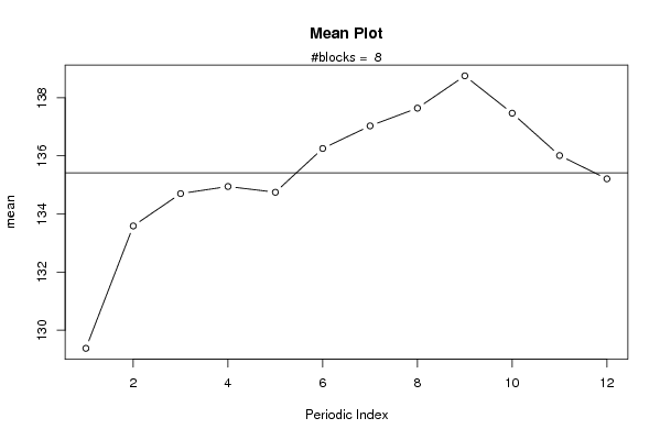
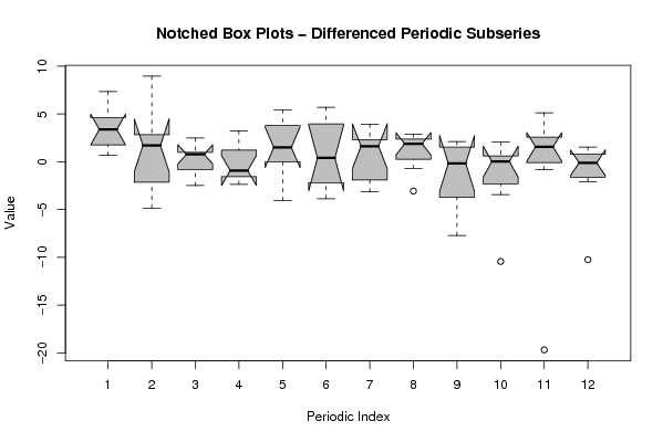
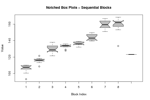
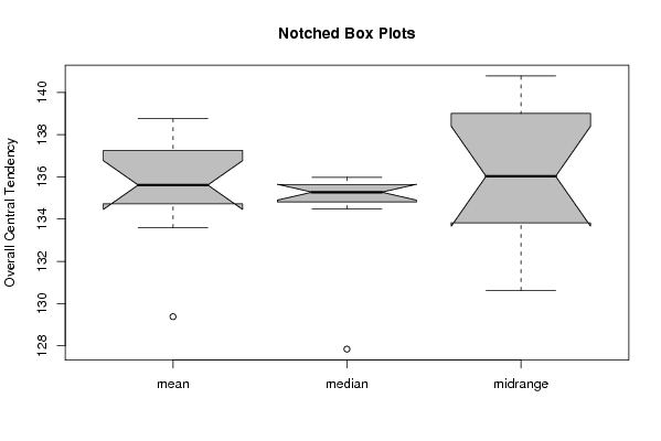
| Title produced by software | Mean Plot | ||||||||||||||||||||
| Date of computation | Wed, 17 Dec 2008 12:23:44 -0700 | ||||||||||||||||||||
| Cite this page as follows | Statistical Computations at FreeStatistics.org, Office for Research Development and Education, URL https://freestatistics.org/blog/index.php?v=date/2008/Dec/17/t12295422359f44keu2u0u8z9p.htm/, Retrieved Sun, 19 May 2024 06:05:30 +0000 | ||||||||||||||||||||
| Statistical Computations at FreeStatistics.org, Office for Research Development and Education, URL https://freestatistics.org/blog/index.php?pk=34512, Retrieved Sun, 19 May 2024 06:05:30 +0000 | |||||||||||||||||||||
| QR Codes: | |||||||||||||||||||||
|
| |||||||||||||||||||||
| Original text written by user: | |||||||||||||||||||||
| IsPrivate? | No (this computation is public) | ||||||||||||||||||||
| User-defined keywords | S0800650 Jan Werkhoven | ||||||||||||||||||||
| Estimated Impact | 163 | ||||||||||||||||||||
Tree of Dependent Computations | |||||||||||||||||||||
| Family? (F = Feedback message, R = changed R code, M = changed R Module, P = changed Parameters, D = changed Data) | |||||||||||||||||||||
| - [Univariate Data Series] [Exchange rate of ...] [2008-12-17 19:18:06] [944cfe91fab3d898afdbc7f6b8914047] - RMPD [Mean Plot] [D4:Mean Plot] [2008-12-17 19:23:44] [721fbc57bdc4e4e6ec78137fe5a723c9] [Current] | |||||||||||||||||||||
| Feedback Forum | |||||||||||||||||||||
Post a new message | |||||||||||||||||||||
Dataset | |||||||||||||||||||||
| Dataseries X: | |||||||||||||||||||||
93.26 100.61 109.57 107.08 110.33 110.36 106.5 104.3 107.21 109.34 108.2 109.86 108.68 113.38 117.12 116.23 114.75 115.81 115.86 117.8 117.11 116.31 118.38 121.57 121.65 124.2 126.12 128.6 128.16 130.12 135.83 138.05 134.99 132.38 128.94 128.12 127.84 132.43 134.13 134.78 133.13 129.08 134.48 132.86 134.08 134.54 134.51 135.97 136.09 139.14 135.63 136.55 138.83 138.84 135.37 132.22 134.75 135.98 136.06 138.05 139.59 140.58 139.81 140.77 140.96 143.59 142.7 145.11 146.7 148.53 148.99 149.65 151.11 154.82 156.56 157.6 155.24 160.68 163.22 164.55 166.76 159.05 159.82 164.95 162.89 163.55 158.68 157.97 156.59 161.56 162.31 166.26 168.45 163.63 153.2 133.52 123.28 | |||||||||||||||||||||
Tables (Output of Computation) | |||||||||||||||||||||
| |||||||||||||||||||||
Figures (Output of Computation) | |||||||||||||||||||||
Input Parameters & R Code | |||||||||||||||||||||
| Parameters (Session): | |||||||||||||||||||||
| par1 = 12 ; | |||||||||||||||||||||
| Parameters (R input): | |||||||||||||||||||||
| par1 = 12 ; | |||||||||||||||||||||
| R code (references can be found in the software module): | |||||||||||||||||||||
par1 <- as.numeric(par1) | |||||||||||||||||||||