Repository of Reproducible Computations

Free Statistics

of Irreproducible Research!

Author's title

Author

*Unverified author*

R Software Module

rwasp_autocorrelation.wasp

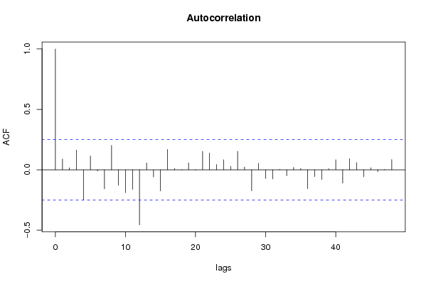
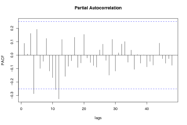
Title produced by software

(Partial) Autocorrelation Function

Date of computation

Wed, 17 Dec 2008 11:47:42 -0700

Cite this page as follows

Statistical Computations at FreeStatistics.org, Office for Research Development and Education, URL https://freestatistics.org/blog/index.php?v=date/2008/Dec/17/t12295396964hdaegwhdjrby73.htm/, Retrieved Mon, 27 May 2024 04:02:28 +0000

Statistical Computations at FreeStatistics.org, Office for Research Development and Education, URL https://freestatistics.org/blog/index.php?pk=34484, Retrieved Mon, 27 May 2024 04:02:28 +0000

QR Codes:

Paste this QR Code to cite your computation.

Original text written by user:

IsPrivate?

No (this computation is public)

User-defined keywords

Estimated Impact

161

Family? (F = Feedback message, R = changed R code, M = changed R Module, P = changed Parameters, D = changed Data)

-     [Standard Deviation-Mean Plot] [TAAK] [2008-12-16 20:59:02] [f3161d5a04a14312cd010aa8f92941cc]
- RM D  [Variance Reduction Matrix] [TAAK] [2008-12-17 18:15:17] [f3161d5a04a14312cd010aa8f92941cc]
- RMPD    [(Partial) Autocorrelation Function] [Taak] [2008-12-17 18:25:12] [f3161d5a04a14312cd010aa8f92941cc]
-   P       [(Partial) Autocorrelation Function] [Taak] [2008-12-17 18:31:00] [f3161d5a04a14312cd010aa8f92941cc]
-   PD        [(Partial) Autocorrelation Function] [Taak] [2008-12-17 18:43:02] [f3161d5a04a14312cd010aa8f92941cc]
-   P           [(Partial) Autocorrelation Function] [Taak] [2008-12-17 18:46:14] [f3161d5a04a14312cd010aa8f92941cc]
-   P               [(Partial) Autocorrelation Function] [Taak] [2008-12-17 18:47:42] [59094f58b9d90d3694e930ebd2901ecd] [Current]

Feedback Forum

Post a new message

Dataseries X:

Download CSV

Histogram

Boxplots

Summary of computational transaction
Raw Input	view raw input (R code)
Raw Output	view raw output of R engine
Computing time	1 seconds
R Server	'Sir Ronald Aylmer Fisher' @ 193.190.124.24

\begin{tabular}{lllllllll}
\hline
Summary of computational transaction \tabularnewline
Raw Input & view raw input (R code)  \tabularnewline
Raw Output & view raw output of R engine  \tabularnewline
Computing time & 1 seconds \tabularnewline
R Server & 'Sir Ronald Aylmer Fisher' @ 193.190.124.24 \tabularnewline
\hline
\end{tabular}
%Source: https://freestatistics.org/blog/index.php?pk=34484&T=0

[TABLE]
[ROW][C]Summary of computational transaction[/C][/ROW]
[ROW][C]Raw Input[/C][C]view raw input (R code) [/C][/ROW]
[ROW][C]Raw Output[/C][C]view raw output of R engine [/C][/ROW]
[ROW][C]Computing time[/C][C]1 seconds[/C][/ROW]
[ROW][C]R Server[/C][C]'Sir Ronald Aylmer Fisher' @ 193.190.124.24[/C][/ROW]
[/TABLE]
Source: https://freestatistics.org/blog/index.php?pk=34484&T=0

Globally Unique Identifier (entire table): ba.freestatistics.org/blog/index.php?pk=34484&T=0

As an alternative you can also use a QR Code:

The GUIDs for individual cells are displayed in the table below:

Summary of computational transaction
Raw Input	view raw input (R code)
Raw Output	view raw output of R engine
Computing time	1 seconds
R Server	'Sir Ronald Aylmer Fisher' @ 193.190.124.24

Autocorrelation Function
Time lag k	ACF(k)	T-STAT	P-value
1	0.088588	0.6919	0.245814
2	0.016481	0.1287	0.449001
3	0.163064	1.2736	0.103823
4	-0.249472	-1.9484	0.027983
5	0.114474	0.8941	0.1874
6	-0.009348	-0.073	0.471017
7	-0.157813	-1.2326	0.111235
8	0.201423	1.5732	0.060427
9	-0.12922	-1.0092	0.158424
10	-0.188521	-1.4724	0.073027
11	-0.162429	-1.2686	0.104699
12	-0.455691	-3.5591	0.000364
13	0.056878	0.4442	0.329223
14	-0.060034	-0.4689	0.320414
15	-0.175263	-1.3689	0.088033
16	0.168342	1.3148	0.096751
17	0.010604	0.0828	0.467133
18	-0.00218	-0.017	0.493234
19	0.05634	0.44	0.330736
20	-0.003877	-0.0303	0.487971
21	0.152262	1.1892	0.119483
22	0.138958	1.0853	0.141031
23	0.043373	0.3388	0.36798
24	0.083413	0.6515	0.258592
25	0.028327	0.2212	0.412821
26	0.15289	1.1941	0.118529
27	0.022051	0.1722	0.431916
28	-0.173853	-1.3578	0.089759
29	0.053478	0.4177	0.338826
30	-0.072233	-0.5642	0.287356
31	-0.076423	-0.5969	0.276397
32	0.003718	0.029	0.488466
33	-0.04968	-0.388	0.349678
34	0.020133	0.1572	0.437786
35	0.01028	0.0803	0.468136
36	-0.156466	-1.222	0.113198
37	-0.055933	-0.4369	0.331881
38	-0.079472	-0.6207	0.268556
39	0.008867	0.0693	0.472506
40	0.083017	0.6484	0.259586
41	-0.110505	-0.8631	0.195739
42	0.091741	0.7165	0.238201
43	0.059504	0.4647	0.321887
44	-0.058256	-0.455	0.325365
45	0.01655	0.1293	0.448787
46	-0.01543	-0.1205	0.452238
47	0.002929	0.0229	0.490911
48	0.085081	0.6645	0.254436

\begin{tabular}{lllllllll}
\hline
Autocorrelation Function \tabularnewline
Time lag k & ACF(k) & T-STAT & P-value \tabularnewline
1 & 0.088588 & 0.6919 & 0.245814 \tabularnewline
2 & 0.016481 & 0.1287 & 0.449001 \tabularnewline
3 & 0.163064 & 1.2736 & 0.103823 \tabularnewline
4 & -0.249472 & -1.9484 & 0.027983 \tabularnewline
5 & 0.114474 & 0.8941 & 0.1874 \tabularnewline
6 & -0.009348 & -0.073 & 0.471017 \tabularnewline
7 & -0.157813 & -1.2326 & 0.111235 \tabularnewline
8 & 0.201423 & 1.5732 & 0.060427 \tabularnewline
9 & -0.12922 & -1.0092 & 0.158424 \tabularnewline
10 & -0.188521 & -1.4724 & 0.073027 \tabularnewline
11 & -0.162429 & -1.2686 & 0.104699 \tabularnewline
12 & -0.455691 & -3.5591 & 0.000364 \tabularnewline
13 & 0.056878 & 0.4442 & 0.329223 \tabularnewline
14 & -0.060034 & -0.4689 & 0.320414 \tabularnewline
15 & -0.175263 & -1.3689 & 0.088033 \tabularnewline
16 & 0.168342 & 1.3148 & 0.096751 \tabularnewline
17 & 0.010604 & 0.0828 & 0.467133 \tabularnewline
18 & -0.00218 & -0.017 & 0.493234 \tabularnewline
19 & 0.05634 & 0.44 & 0.330736 \tabularnewline
20 & -0.003877 & -0.0303 & 0.487971 \tabularnewline
21 & 0.152262 & 1.1892 & 0.119483 \tabularnewline
22 & 0.138958 & 1.0853 & 0.141031 \tabularnewline
23 & 0.043373 & 0.3388 & 0.36798 \tabularnewline
24 & 0.083413 & 0.6515 & 0.258592 \tabularnewline
25 & 0.028327 & 0.2212 & 0.412821 \tabularnewline
26 & 0.15289 & 1.1941 & 0.118529 \tabularnewline
27 & 0.022051 & 0.1722 & 0.431916 \tabularnewline
28 & -0.173853 & -1.3578 & 0.089759 \tabularnewline
29 & 0.053478 & 0.4177 & 0.338826 \tabularnewline
30 & -0.072233 & -0.5642 & 0.287356 \tabularnewline
31 & -0.076423 & -0.5969 & 0.276397 \tabularnewline
32 & 0.003718 & 0.029 & 0.488466 \tabularnewline
33 & -0.04968 & -0.388 & 0.349678 \tabularnewline
34 & 0.020133 & 0.1572 & 0.437786 \tabularnewline
35 & 0.01028 & 0.0803 & 0.468136 \tabularnewline
36 & -0.156466 & -1.222 & 0.113198 \tabularnewline
37 & -0.055933 & -0.4369 & 0.331881 \tabularnewline
38 & -0.079472 & -0.6207 & 0.268556 \tabularnewline
39 & 0.008867 & 0.0693 & 0.472506 \tabularnewline
40 & 0.083017 & 0.6484 & 0.259586 \tabularnewline
41 & -0.110505 & -0.8631 & 0.195739 \tabularnewline
42 & 0.091741 & 0.7165 & 0.238201 \tabularnewline
43 & 0.059504 & 0.4647 & 0.321887 \tabularnewline
44 & -0.058256 & -0.455 & 0.325365 \tabularnewline
45 & 0.01655 & 0.1293 & 0.448787 \tabularnewline
46 & -0.01543 & -0.1205 & 0.452238 \tabularnewline
47 & 0.002929 & 0.0229 & 0.490911 \tabularnewline
48 & 0.085081 & 0.6645 & 0.254436 \tabularnewline
\hline
\end{tabular}
%Source: https://freestatistics.org/blog/index.php?pk=34484&T=1

[TABLE]
[ROW][C]Autocorrelation Function[/C][/ROW]
[ROW][C]Time lag k[/C][C]ACF(k)[/C][C]T-STAT[/C][C]P-value[/C][/ROW]
[ROW][C]1[/C][C]0.088588[/C][C]0.6919[/C][C]0.245814[/C][/ROW]
[ROW][C]2[/C][C]0.016481[/C][C]0.1287[/C][C]0.449001[/C][/ROW]
[ROW][C]3[/C][C]0.163064[/C][C]1.2736[/C][C]0.103823[/C][/ROW]
[ROW][C]4[/C][C]-0.249472[/C][C]-1.9484[/C][C]0.027983[/C][/ROW]
[ROW][C]5[/C][C]0.114474[/C][C]0.8941[/C][C]0.1874[/C][/ROW]
[ROW][C]6[/C][C]-0.009348[/C][C]-0.073[/C][C]0.471017[/C][/ROW]
[ROW][C]7[/C][C]-0.157813[/C][C]-1.2326[/C][C]0.111235[/C][/ROW]
[ROW][C]8[/C][C]0.201423[/C][C]1.5732[/C][C]0.060427[/C][/ROW]
[ROW][C]9[/C][C]-0.12922[/C][C]-1.0092[/C][C]0.158424[/C][/ROW]
[ROW][C]10[/C][C]-0.188521[/C][C]-1.4724[/C][C]0.073027[/C][/ROW]
[ROW][C]11[/C][C]-0.162429[/C][C]-1.2686[/C][C]0.104699[/C][/ROW]
[ROW][C]12[/C][C]-0.455691[/C][C]-3.5591[/C][C]0.000364[/C][/ROW]
[ROW][C]13[/C][C]0.056878[/C][C]0.4442[/C][C]0.329223[/C][/ROW]
[ROW][C]14[/C][C]-0.060034[/C][C]-0.4689[/C][C]0.320414[/C][/ROW]
[ROW][C]15[/C][C]-0.175263[/C][C]-1.3689[/C][C]0.088033[/C][/ROW]
[ROW][C]16[/C][C]0.168342[/C][C]1.3148[/C][C]0.096751[/C][/ROW]
[ROW][C]17[/C][C]0.010604[/C][C]0.0828[/C][C]0.467133[/C][/ROW]
[ROW][C]18[/C][C]-0.00218[/C][C]-0.017[/C][C]0.493234[/C][/ROW]
[ROW][C]19[/C][C]0.05634[/C][C]0.44[/C][C]0.330736[/C][/ROW]
[ROW][C]20[/C][C]-0.003877[/C][C]-0.0303[/C][C]0.487971[/C][/ROW]
[ROW][C]21[/C][C]0.152262[/C][C]1.1892[/C][C]0.119483[/C][/ROW]
[ROW][C]22[/C][C]0.138958[/C][C]1.0853[/C][C]0.141031[/C][/ROW]
[ROW][C]23[/C][C]0.043373[/C][C]0.3388[/C][C]0.36798[/C][/ROW]
[ROW][C]24[/C][C]0.083413[/C][C]0.6515[/C][C]0.258592[/C][/ROW]
[ROW][C]25[/C][C]0.028327[/C][C]0.2212[/C][C]0.412821[/C][/ROW]
[ROW][C]26[/C][C]0.15289[/C][C]1.1941[/C][C]0.118529[/C][/ROW]
[ROW][C]27[/C][C]0.022051[/C][C]0.1722[/C][C]0.431916[/C][/ROW]
[ROW][C]28[/C][C]-0.173853[/C][C]-1.3578[/C][C]0.089759[/C][/ROW]
[ROW][C]29[/C][C]0.053478[/C][C]0.4177[/C][C]0.338826[/C][/ROW]
[ROW][C]30[/C][C]-0.072233[/C][C]-0.5642[/C][C]0.287356[/C][/ROW]
[ROW][C]31[/C][C]-0.076423[/C][C]-0.5969[/C][C]0.276397[/C][/ROW]
[ROW][C]32[/C][C]0.003718[/C][C]0.029[/C][C]0.488466[/C][/ROW]
[ROW][C]33[/C][C]-0.04968[/C][C]-0.388[/C][C]0.349678[/C][/ROW]
[ROW][C]34[/C][C]0.020133[/C][C]0.1572[/C][C]0.437786[/C][/ROW]
[ROW][C]35[/C][C]0.01028[/C][C]0.0803[/C][C]0.468136[/C][/ROW]
[ROW][C]36[/C][C]-0.156466[/C][C]-1.222[/C][C]0.113198[/C][/ROW]
[ROW][C]37[/C][C]-0.055933[/C][C]-0.4369[/C][C]0.331881[/C][/ROW]
[ROW][C]38[/C][C]-0.079472[/C][C]-0.6207[/C][C]0.268556[/C][/ROW]
[ROW][C]39[/C][C]0.008867[/C][C]0.0693[/C][C]0.472506[/C][/ROW]
[ROW][C]40[/C][C]0.083017[/C][C]0.6484[/C][C]0.259586[/C][/ROW]
[ROW][C]41[/C][C]-0.110505[/C][C]-0.8631[/C][C]0.195739[/C][/ROW]
[ROW][C]42[/C][C]0.091741[/C][C]0.7165[/C][C]0.238201[/C][/ROW]
[ROW][C]43[/C][C]0.059504[/C][C]0.4647[/C][C]0.321887[/C][/ROW]
[ROW][C]44[/C][C]-0.058256[/C][C]-0.455[/C][C]0.325365[/C][/ROW]
[ROW][C]45[/C][C]0.01655[/C][C]0.1293[/C][C]0.448787[/C][/ROW]
[ROW][C]46[/C][C]-0.01543[/C][C]-0.1205[/C][C]0.452238[/C][/ROW]
[ROW][C]47[/C][C]0.002929[/C][C]0.0229[/C][C]0.490911[/C][/ROW]
[ROW][C]48[/C][C]0.085081[/C][C]0.6645[/C][C]0.254436[/C][/ROW]
[/TABLE]
Source: https://freestatistics.org/blog/index.php?pk=34484&T=1

Globally Unique Identifier (entire table): ba.freestatistics.org/blog/index.php?pk=34484&T=1

As an alternative you can also use a QR Code:

The GUIDs for individual cells are displayed in the table below:

Autocorrelation Function
Time lag k	ACF(k)	T-STAT	P-value
1	0.088588	0.6919	0.245814
2	0.016481	0.1287	0.449001
3	0.163064	1.2736	0.103823
4	-0.249472	-1.9484	0.027983
5	0.114474	0.8941	0.1874
6	-0.009348	-0.073	0.471017
7	-0.157813	-1.2326	0.111235
8	0.201423	1.5732	0.060427
9	-0.12922	-1.0092	0.158424
10	-0.188521	-1.4724	0.073027
11	-0.162429	-1.2686	0.104699
12	-0.455691	-3.5591	0.000364
13	0.056878	0.4442	0.329223
14	-0.060034	-0.4689	0.320414
15	-0.175263	-1.3689	0.088033
16	0.168342	1.3148	0.096751
17	0.010604	0.0828	0.467133
18	-0.00218	-0.017	0.493234
19	0.05634	0.44	0.330736
20	-0.003877	-0.0303	0.487971
21	0.152262	1.1892	0.119483
22	0.138958	1.0853	0.141031
23	0.043373	0.3388	0.36798
24	0.083413	0.6515	0.258592
25	0.028327	0.2212	0.412821
26	0.15289	1.1941	0.118529
27	0.022051	0.1722	0.431916
28	-0.173853	-1.3578	0.089759
29	0.053478	0.4177	0.338826
30	-0.072233	-0.5642	0.287356
31	-0.076423	-0.5969	0.276397
32	0.003718	0.029	0.488466
33	-0.04968	-0.388	0.349678
34	0.020133	0.1572	0.437786
35	0.01028	0.0803	0.468136
36	-0.156466	-1.222	0.113198
37	-0.055933	-0.4369	0.331881
38	-0.079472	-0.6207	0.268556
39	0.008867	0.0693	0.472506
40	0.083017	0.6484	0.259586
41	-0.110505	-0.8631	0.195739
42	0.091741	0.7165	0.238201
43	0.059504	0.4647	0.321887
44	-0.058256	-0.455	0.325365
45	0.01655	0.1293	0.448787
46	-0.01543	-0.1205	0.452238
47	0.002929	0.0229	0.490911
48	0.085081	0.6645	0.254436

Partial Autocorrelation Function
Time lag k	PACF(k)	T-STAT	P-value
1	0.088588	0.6919	0.245814
2	0.008702	0.068	0.473019
3	0.162131	1.2663	0.105114
4	-0.287613	-2.2463	0.014157
5	0.193234	1.5092	0.068204
6	-0.098946	-0.7728	0.221315
7	-0.045779	-0.3575	0.360958
8	0.125189	0.9778	0.166029
9	-0.118072	-0.9222	0.180036
10	-0.167435	-1.3077	0.097939
11	-0.256943	-2.0068	0.024605
12	-0.326264	-2.5482	0.006681
13	0.117546	0.9181	0.181101
14	-0.158267	-1.2361	0.110579
15	-0.08277	-0.6465	0.260204
16	-0.041593	-0.3249	0.373202
17	0.133706	1.0443	0.15024
18	-0.091818	-0.7171	0.238018
19	-0.058133	-0.454	0.325708
20	0.155077	1.2112	0.115247
21	-0.020401	-0.1593	0.436966
22	-0.054442	-0.4252	0.336093
23	-0.077341	-0.6041	0.274024
24	-0.089497	-0.699	0.243607
25	0.039564	0.309	0.379186
26	0.082684	0.6458	0.260421
27	-0.038889	-0.3037	0.381183
28	-0.148986	-1.1636	0.124555
29	0.11832	0.9241	0.179536
30	-0.118777	-0.9277	0.178615
31	0.017847	0.1394	0.444802
32	0.083132	0.6493	0.259296
33	0.101959	0.7963	0.214465
34	-0.052445	-0.4096	0.341765
35	0.038312	0.2992	0.382892
36	-0.10586	-0.8268	0.205789
37	0.004609	0.036	0.4857
38	-0.059399	-0.4639	0.322177
39	0.002181	0.017	0.493233
40	-0.086903	-0.6787	0.249938
41	-0.046532	-0.3634	0.358771
42	-0.073766	-0.5761	0.283323
43	-0.000155	-0.0012	0.499518
44	0.090217	0.7046	0.241865
45	-0.025847	-0.2019	0.420344
46	-0.060066	-0.4691	0.320325
47	-0.026115	-0.204	0.41953
48	-0.075587	-0.5904	0.278568

\begin{tabular}{lllllllll}
\hline
Partial Autocorrelation Function \tabularnewline
Time lag k & PACF(k) & T-STAT & P-value \tabularnewline
1 & 0.088588 & 0.6919 & 0.245814 \tabularnewline
2 & 0.008702 & 0.068 & 0.473019 \tabularnewline
3 & 0.162131 & 1.2663 & 0.105114 \tabularnewline
4 & -0.287613 & -2.2463 & 0.014157 \tabularnewline
5 & 0.193234 & 1.5092 & 0.068204 \tabularnewline
6 & -0.098946 & -0.7728 & 0.221315 \tabularnewline
7 & -0.045779 & -0.3575 & 0.360958 \tabularnewline
8 & 0.125189 & 0.9778 & 0.166029 \tabularnewline
9 & -0.118072 & -0.9222 & 0.180036 \tabularnewline
10 & -0.167435 & -1.3077 & 0.097939 \tabularnewline
11 & -0.256943 & -2.0068 & 0.024605 \tabularnewline
12 & -0.326264 & -2.5482 & 0.006681 \tabularnewline
13 & 0.117546 & 0.9181 & 0.181101 \tabularnewline
14 & -0.158267 & -1.2361 & 0.110579 \tabularnewline
15 & -0.08277 & -0.6465 & 0.260204 \tabularnewline
16 & -0.041593 & -0.3249 & 0.373202 \tabularnewline
17 & 0.133706 & 1.0443 & 0.15024 \tabularnewline
18 & -0.091818 & -0.7171 & 0.238018 \tabularnewline
19 & -0.058133 & -0.454 & 0.325708 \tabularnewline
20 & 0.155077 & 1.2112 & 0.115247 \tabularnewline
21 & -0.020401 & -0.1593 & 0.436966 \tabularnewline
22 & -0.054442 & -0.4252 & 0.336093 \tabularnewline
23 & -0.077341 & -0.6041 & 0.274024 \tabularnewline
24 & -0.089497 & -0.699 & 0.243607 \tabularnewline
25 & 0.039564 & 0.309 & 0.379186 \tabularnewline
26 & 0.082684 & 0.6458 & 0.260421 \tabularnewline
27 & -0.038889 & -0.3037 & 0.381183 \tabularnewline
28 & -0.148986 & -1.1636 & 0.124555 \tabularnewline
29 & 0.11832 & 0.9241 & 0.179536 \tabularnewline
30 & -0.118777 & -0.9277 & 0.178615 \tabularnewline
31 & 0.017847 & 0.1394 & 0.444802 \tabularnewline
32 & 0.083132 & 0.6493 & 0.259296 \tabularnewline
33 & 0.101959 & 0.7963 & 0.214465 \tabularnewline
34 & -0.052445 & -0.4096 & 0.341765 \tabularnewline
35 & 0.038312 & 0.2992 & 0.382892 \tabularnewline
36 & -0.10586 & -0.8268 & 0.205789 \tabularnewline
37 & 0.004609 & 0.036 & 0.4857 \tabularnewline
38 & -0.059399 & -0.4639 & 0.322177 \tabularnewline
39 & 0.002181 & 0.017 & 0.493233 \tabularnewline
40 & -0.086903 & -0.6787 & 0.249938 \tabularnewline
41 & -0.046532 & -0.3634 & 0.358771 \tabularnewline
42 & -0.073766 & -0.5761 & 0.283323 \tabularnewline
43 & -0.000155 & -0.0012 & 0.499518 \tabularnewline
44 & 0.090217 & 0.7046 & 0.241865 \tabularnewline
45 & -0.025847 & -0.2019 & 0.420344 \tabularnewline
46 & -0.060066 & -0.4691 & 0.320325 \tabularnewline
47 & -0.026115 & -0.204 & 0.41953 \tabularnewline
48 & -0.075587 & -0.5904 & 0.278568 \tabularnewline
\hline
\end{tabular}
%Source: https://freestatistics.org/blog/index.php?pk=34484&T=2

[TABLE]
[ROW][C]Partial Autocorrelation Function[/C][/ROW]
[ROW][C]Time lag k[/C][C]PACF(k)[/C][C]T-STAT[/C][C]P-value[/C][/ROW]
[ROW][C]1[/C][C]0.088588[/C][C]0.6919[/C][C]0.245814[/C][/ROW]
[ROW][C]2[/C][C]0.008702[/C][C]0.068[/C][C]0.473019[/C][/ROW]
[ROW][C]3[/C][C]0.162131[/C][C]1.2663[/C][C]0.105114[/C][/ROW]
[ROW][C]4[/C][C]-0.287613[/C][C]-2.2463[/C][C]0.014157[/C][/ROW]
[ROW][C]5[/C][C]0.193234[/C][C]1.5092[/C][C]0.068204[/C][/ROW]
[ROW][C]6[/C][C]-0.098946[/C][C]-0.7728[/C][C]0.221315[/C][/ROW]
[ROW][C]7[/C][C]-0.045779[/C][C]-0.3575[/C][C]0.360958[/C][/ROW]
[ROW][C]8[/C][C]0.125189[/C][C]0.9778[/C][C]0.166029[/C][/ROW]
[ROW][C]9[/C][C]-0.118072[/C][C]-0.9222[/C][C]0.180036[/C][/ROW]
[ROW][C]10[/C][C]-0.167435[/C][C]-1.3077[/C][C]0.097939[/C][/ROW]
[ROW][C]11[/C][C]-0.256943[/C][C]-2.0068[/C][C]0.024605[/C][/ROW]
[ROW][C]12[/C][C]-0.326264[/C][C]-2.5482[/C][C]0.006681[/C][/ROW]
[ROW][C]13[/C][C]0.117546[/C][C]0.9181[/C][C]0.181101[/C][/ROW]
[ROW][C]14[/C][C]-0.158267[/C][C]-1.2361[/C][C]0.110579[/C][/ROW]
[ROW][C]15[/C][C]-0.08277[/C][C]-0.6465[/C][C]0.260204[/C][/ROW]
[ROW][C]16[/C][C]-0.041593[/C][C]-0.3249[/C][C]0.373202[/C][/ROW]
[ROW][C]17[/C][C]0.133706[/C][C]1.0443[/C][C]0.15024[/C][/ROW]
[ROW][C]18[/C][C]-0.091818[/C][C]-0.7171[/C][C]0.238018[/C][/ROW]
[ROW][C]19[/C][C]-0.058133[/C][C]-0.454[/C][C]0.325708[/C][/ROW]
[ROW][C]20[/C][C]0.155077[/C][C]1.2112[/C][C]0.115247[/C][/ROW]
[ROW][C]21[/C][C]-0.020401[/C][C]-0.1593[/C][C]0.436966[/C][/ROW]
[ROW][C]22[/C][C]-0.054442[/C][C]-0.4252[/C][C]0.336093[/C][/ROW]
[ROW][C]23[/C][C]-0.077341[/C][C]-0.6041[/C][C]0.274024[/C][/ROW]
[ROW][C]24[/C][C]-0.089497[/C][C]-0.699[/C][C]0.243607[/C][/ROW]
[ROW][C]25[/C][C]0.039564[/C][C]0.309[/C][C]0.379186[/C][/ROW]
[ROW][C]26[/C][C]0.082684[/C][C]0.6458[/C][C]0.260421[/C][/ROW]
[ROW][C]27[/C][C]-0.038889[/C][C]-0.3037[/C][C]0.381183[/C][/ROW]
[ROW][C]28[/C][C]-0.148986[/C][C]-1.1636[/C][C]0.124555[/C][/ROW]
[ROW][C]29[/C][C]0.11832[/C][C]0.9241[/C][C]0.179536[/C][/ROW]
[ROW][C]30[/C][C]-0.118777[/C][C]-0.9277[/C][C]0.178615[/C][/ROW]
[ROW][C]31[/C][C]0.017847[/C][C]0.1394[/C][C]0.444802[/C][/ROW]
[ROW][C]32[/C][C]0.083132[/C][C]0.6493[/C][C]0.259296[/C][/ROW]
[ROW][C]33[/C][C]0.101959[/C][C]0.7963[/C][C]0.214465[/C][/ROW]
[ROW][C]34[/C][C]-0.052445[/C][C]-0.4096[/C][C]0.341765[/C][/ROW]
[ROW][C]35[/C][C]0.038312[/C][C]0.2992[/C][C]0.382892[/C][/ROW]
[ROW][C]36[/C][C]-0.10586[/C][C]-0.8268[/C][C]0.205789[/C][/ROW]
[ROW][C]37[/C][C]0.004609[/C][C]0.036[/C][C]0.4857[/C][/ROW]
[ROW][C]38[/C][C]-0.059399[/C][C]-0.4639[/C][C]0.322177[/C][/ROW]
[ROW][C]39[/C][C]0.002181[/C][C]0.017[/C][C]0.493233[/C][/ROW]
[ROW][C]40[/C][C]-0.086903[/C][C]-0.6787[/C][C]0.249938[/C][/ROW]
[ROW][C]41[/C][C]-0.046532[/C][C]-0.3634[/C][C]0.358771[/C][/ROW]
[ROW][C]42[/C][C]-0.073766[/C][C]-0.5761[/C][C]0.283323[/C][/ROW]
[ROW][C]43[/C][C]-0.000155[/C][C]-0.0012[/C][C]0.499518[/C][/ROW]
[ROW][C]44[/C][C]0.090217[/C][C]0.7046[/C][C]0.241865[/C][/ROW]
[ROW][C]45[/C][C]-0.025847[/C][C]-0.2019[/C][C]0.420344[/C][/ROW]
[ROW][C]46[/C][C]-0.060066[/C][C]-0.4691[/C][C]0.320325[/C][/ROW]
[ROW][C]47[/C][C]-0.026115[/C][C]-0.204[/C][C]0.41953[/C][/ROW]
[ROW][C]48[/C][C]-0.075587[/C][C]-0.5904[/C][C]0.278568[/C][/ROW]
[/TABLE]
Source: https://freestatistics.org/blog/index.php?pk=34484&T=2

Globally Unique Identifier (entire table): ba.freestatistics.org/blog/index.php?pk=34484&T=2

As an alternative you can also use a QR Code:

The GUIDs for individual cells are displayed in the table below:

Partial Autocorrelation Function
Time lag k	PACF(k)	T-STAT	P-value
1	0.088588	0.6919	0.245814
2	0.008702	0.068	0.473019
3	0.162131	1.2663	0.105114
4	-0.287613	-2.2463	0.014157
5	0.193234	1.5092	0.068204
6	-0.098946	-0.7728	0.221315
7	-0.045779	-0.3575	0.360958
8	0.125189	0.9778	0.166029
9	-0.118072	-0.9222	0.180036
10	-0.167435	-1.3077	0.097939
11	-0.256943	-2.0068	0.024605
12	-0.326264	-2.5482	0.006681
13	0.117546	0.9181	0.181101
14	-0.158267	-1.2361	0.110579
15	-0.08277	-0.6465	0.260204
16	-0.041593	-0.3249	0.373202
17	0.133706	1.0443	0.15024
18	-0.091818	-0.7171	0.238018
19	-0.058133	-0.454	0.325708
20	0.155077	1.2112	0.115247
21	-0.020401	-0.1593	0.436966
22	-0.054442	-0.4252	0.336093
23	-0.077341	-0.6041	0.274024
24	-0.089497	-0.699	0.243607
25	0.039564	0.309	0.379186
26	0.082684	0.6458	0.260421
27	-0.038889	-0.3037	0.381183
28	-0.148986	-1.1636	0.124555
29	0.11832	0.9241	0.179536
30	-0.118777	-0.9277	0.178615
31	0.017847	0.1394	0.444802
32	0.083132	0.6493	0.259296
33	0.101959	0.7963	0.214465
34	-0.052445	-0.4096	0.341765
35	0.038312	0.2992	0.382892
36	-0.10586	-0.8268	0.205789
37	0.004609	0.036	0.4857
38	-0.059399	-0.4639	0.322177
39	0.002181	0.017	0.493233
40	-0.086903	-0.6787	0.249938
41	-0.046532	-0.3634	0.358771
42	-0.073766	-0.5761	0.283323
43	-0.000155	-0.0012	0.499518
44	0.090217	0.7046	0.241865
45	-0.025847	-0.2019	0.420344
46	-0.060066	-0.4691	0.320325
47	-0.026115	-0.204	0.41953
48	-0.075587	-0.5904	0.278568

Figure 1

PNG link

Postscript link

PDF link

Figure 2

PNG link

Postscript link

PDF link

Parameters (Session):

par1 = 48 ; par2 = 1 ; par3 = 1 ; par4 = 1 ; par5 = 12 ;

Parameters (R input):

par1 = 48 ; par2 = 1 ; par3 = 1 ; par4 = 1 ; par5 = 12 ;

R code (references can be found in the software module):

if (par1 == 'Default') {
par1 = 10*log10(length(x))
} else {
par1 <- as.numeric(par1)
}
par2 <- as.numeric(par2)
par3 <- as.numeric(par3)
par4 <- as.numeric(par4)
par5 <- as.numeric(par5)
if (par2 == 0) {
x <- log(x)
} else {
x <- (x ^ par2 - 1) / par2
}
if (par3 > 0) x <- diff(x,lag=1,difference=par3)
if (par4 > 0) x <- diff(x,lag=par5,difference=par4)
bitmap(file='pic1.png')
racf <- acf(x,par1,main='Autocorrelation',xlab='lags',ylab='ACF')
dev.off()
bitmap(file='pic2.png')
rpacf <- pacf(x,par1,main='Partial Autocorrelation',xlab='lags',ylab='PACF')
dev.off()
(myacf <- c(racf$acf))
(mypacf <- c(rpacf$acf))
lengthx <- length(x)
sqrtn <- sqrt(lengthx)
load(file='createtable')
a<-table.start()
a<-table.row.start(a)
a<-table.element(a,'Autocorrelation Function',4,TRUE)
a<-table.row.end(a)
a<-table.row.start(a)
a<-table.element(a,'Time lag k',header=TRUE)
a<-table.element(a,hyperlink('basics.htm','ACF(k)','click here for more information about the Autocorrelation Function'),header=TRUE)
a<-table.element(a,'T-STAT',header=TRUE)
a<-table.element(a,'P-value',header=TRUE)
a<-table.row.end(a)
for (i in 2:(par1+1)) {
a<-table.row.start(a)
a<-table.element(a,i-1,header=TRUE)
a<-table.element(a,round(myacf[i],6))
mytstat <- myacf[i]*sqrtn
a<-table.element(a,round(mytstat,4))
a<-table.element(a,round(1-pt(abs(mytstat),lengthx),6))
a<-table.row.end(a)
}
a<-table.end(a)
table.save(a,file='mytable.tab')
a<-table.start()
a<-table.row.start(a)
a<-table.element(a,'Partial Autocorrelation Function',4,TRUE)
a<-table.row.end(a)
a<-table.row.start(a)
a<-table.element(a,'Time lag k',header=TRUE)
a<-table.element(a,hyperlink('basics.htm','PACF(k)','click here for more information about the Partial Autocorrelation Function'),header=TRUE)
a<-table.element(a,'T-STAT',header=TRUE)
a<-table.element(a,'P-value',header=TRUE)
a<-table.row.end(a)
for (i in 1:par1) {
a<-table.row.start(a)
a<-table.element(a,i,header=TRUE)
a<-table.element(a,round(mypacf[i],6))
mytstat <- mypacf[i]*sqrtn
a<-table.element(a,round(mytstat,4))
a<-table.element(a,round(1-pt(abs(mytstat),lengthx),6))
a<-table.row.end(a)
}
a<-table.end(a)
table.save(a,file='mytable1.tab')

Free Statistics

Description of Statistical Computation

Tree of Dependent Computations

Dataset

Tables (Output of Computation)

Figures (Output of Computation)

Input Parameters & R Code