Repository of Reproducible Computations

Free Statistics

of Irreproducible Research!

Author's title

Author

*Unverified author*

R Software Module

rwasp_autocorrelation.wasp

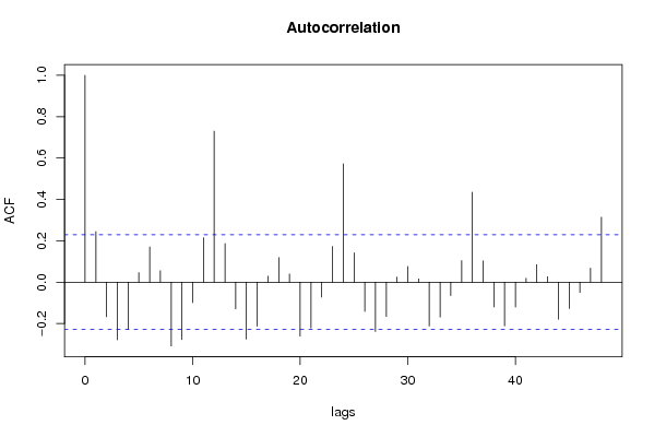
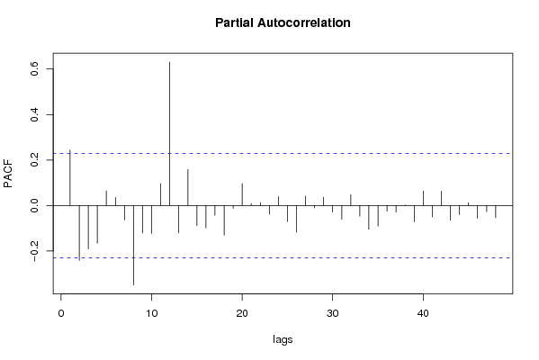
Title produced by software

(Partial) Autocorrelation Function

Date of computation

Wed, 17 Dec 2008 11:31:00 -0700

Cite this page as follows

Statistical Computations at FreeStatistics.org, Office for Research Development and Education, URL https://freestatistics.org/blog/index.php?v=date/2008/Dec/17/t1229538685aa8dcqbkq8zp29j.htm/, Retrieved Sun, 19 May 2024 06:28:16 +0000

Statistical Computations at FreeStatistics.org, Office for Research Development and Education, URL https://freestatistics.org/blog/index.php?pk=34477, Retrieved Sun, 19 May 2024 06:28:16 +0000

QR Codes:

Paste this QR Code to cite your computation.

Original text written by user:

IsPrivate?

No (this computation is public)

User-defined keywords

Estimated Impact

152

Family? (F = Feedback message, R = changed R code, M = changed R Module, P = changed Parameters, D = changed Data)

-     [Standard Deviation-Mean Plot] [TAAK] [2008-12-16 20:59:02] [f3161d5a04a14312cd010aa8f92941cc]
- RM D  [Variance Reduction Matrix] [TAAK] [2008-12-17 18:15:17] [f3161d5a04a14312cd010aa8f92941cc]
- RMPD    [(Partial) Autocorrelation Function] [Taak] [2008-12-17 18:25:12] [f3161d5a04a14312cd010aa8f92941cc]
-   P         [(Partial) Autocorrelation Function] [Taak] [2008-12-17 18:31:00] [59094f58b9d90d3694e930ebd2901ecd] [Current]
-   P           [(Partial) Autocorrelation Function] [Taak] [2008-12-17 18:33:23] [f3161d5a04a14312cd010aa8f92941cc] 
-   PD          [(Partial) Autocorrelation Function] [Taak] [2008-12-17 18:43:02] [f3161d5a04a14312cd010aa8f92941cc] 
-   P             [(Partial) Autocorrelation Function] [Taak] [2008-12-17 18:46:14] [f3161d5a04a14312cd010aa8f92941cc] 
-   P               [(Partial) Autocorrelation Function] [Taak] [2008-12-17 18:47:42] [f3161d5a04a14312cd010aa8f92941cc] 
- RMP               [Spectral Analysis] [Taak] [2008-12-17 18:53:33] [f3161d5a04a14312cd010aa8f92941cc] 
-                     [Spectral Analysis] [Taak] [2008-12-17 18:55:19] [f3161d5a04a14312cd010aa8f92941cc] 

Feedback Forum

Post a new message

Dataseries X:

Download CSV

Histogram

Boxplots

Summary of computational transaction
Raw Input	view raw input (R code)
Raw Output	view raw output of R engine
Computing time	1 seconds
R Server	'Gwilym Jenkins' @ 72.249.127.135

\begin{tabular}{lllllllll}
\hline
Summary of computational transaction \tabularnewline
Raw Input & view raw input (R code)  \tabularnewline
Raw Output & view raw output of R engine  \tabularnewline
Computing time & 1 seconds \tabularnewline
R Server & 'Gwilym Jenkins' @ 72.249.127.135 \tabularnewline
\hline
\end{tabular}
%Source: https://freestatistics.org/blog/index.php?pk=34477&T=0

[TABLE]
[ROW][C]Summary of computational transaction[/C][/ROW]
[ROW][C]Raw Input[/C][C]view raw input (R code) [/C][/ROW]
[ROW][C]Raw Output[/C][C]view raw output of R engine [/C][/ROW]
[ROW][C]Computing time[/C][C]1 seconds[/C][/ROW]
[ROW][C]R Server[/C][C]'Gwilym Jenkins' @ 72.249.127.135[/C][/ROW]
[/TABLE]
Source: https://freestatistics.org/blog/index.php?pk=34477&T=0

Globally Unique Identifier (entire table): ba.freestatistics.org/blog/index.php?pk=34477&T=0

As an alternative you can also use a QR Code:

The GUIDs for individual cells are displayed in the table below:

Summary of computational transaction
Raw Input	view raw input (R code)
Raw Output	view raw output of R engine
Computing time	1 seconds
R Server	'Gwilym Jenkins' @ 72.249.127.135

Autocorrelation Function
Time lag k	ACF(k)	T-STAT	P-value
1	0.243769	2.0828	0.020388
2	-0.167359	-1.4299	0.078503
3	-0.278663	-2.3809	0.00994
4	-0.228896	-1.9557	0.027165
5	0.045981	0.3929	0.347784
6	0.170263	1.4547	0.075016
7	0.055364	0.473	0.318802
8	-0.308419	-2.6351	0.005133
9	-0.277549	-2.3714	0.010181
10	-0.098362	-0.8404	0.201714
11	0.214995	1.8369	0.035146
12	0.729937	6.2366	0
13	0.186383	1.5925	0.057802
14	-0.129118	-1.1032	0.136786
15	-0.275411	-2.3531	0.010657
16	-0.212718	-1.8175	0.036625
17	0.028576	0.2442	0.403899
18	0.118507	1.0125	0.157315
19	0.039309	0.3359	0.368973
20	-0.261369	-2.2331	0.014303
21	-0.221253	-1.8904	0.031338
22	-0.072179	-0.6167	0.269676
23	0.17279	1.4763	0.07208
24	0.572015	4.8873	3e-06
25	0.141942	1.2128	0.114567
26	-0.141504	-1.209	0.11528
27	-0.238429	-2.0371	0.022631
28	-0.165859	-1.4171	0.080354
29	0.024514	0.2094	0.417342
30	0.075947	0.6489	0.259222
31	0.015658	0.1338	0.446971
32	-0.212222	-1.8132	0.036954
33	-0.168418	-1.439	0.077218
34	-0.064829	-0.5539	0.290671
35	0.104131	0.8897	0.188275
36	0.435049	3.7171	0.000196
37	0.102476	0.8756	0.192071
38	-0.120002	-1.0253	0.154304
39	-0.211838	-1.8099	0.03721
40	-0.120723	-1.0315	0.152865
41	0.018613	0.159	0.437042
42	0.085193	0.7279	0.234504
43	0.025912	0.2214	0.412703
44	-0.178996	-1.5293	0.065251
45	-0.127156	-1.0864	0.140434
46	-0.050363	-0.4303	0.334122
47	0.067446	0.5763	0.283107
48	0.31392	2.6821	0.004521

\begin{tabular}{lllllllll}
\hline
Autocorrelation Function \tabularnewline
Time lag k & ACF(k) & T-STAT & P-value \tabularnewline
1 & 0.243769 & 2.0828 & 0.020388 \tabularnewline
2 & -0.167359 & -1.4299 & 0.078503 \tabularnewline
3 & -0.278663 & -2.3809 & 0.00994 \tabularnewline
4 & -0.228896 & -1.9557 & 0.027165 \tabularnewline
5 & 0.045981 & 0.3929 & 0.347784 \tabularnewline
6 & 0.170263 & 1.4547 & 0.075016 \tabularnewline
7 & 0.055364 & 0.473 & 0.318802 \tabularnewline
8 & -0.308419 & -2.6351 & 0.005133 \tabularnewline
9 & -0.277549 & -2.3714 & 0.010181 \tabularnewline
10 & -0.098362 & -0.8404 & 0.201714 \tabularnewline
11 & 0.214995 & 1.8369 & 0.035146 \tabularnewline
12 & 0.729937 & 6.2366 & 0 \tabularnewline
13 & 0.186383 & 1.5925 & 0.057802 \tabularnewline
14 & -0.129118 & -1.1032 & 0.136786 \tabularnewline
15 & -0.275411 & -2.3531 & 0.010657 \tabularnewline
16 & -0.212718 & -1.8175 & 0.036625 \tabularnewline
17 & 0.028576 & 0.2442 & 0.403899 \tabularnewline
18 & 0.118507 & 1.0125 & 0.157315 \tabularnewline
19 & 0.039309 & 0.3359 & 0.368973 \tabularnewline
20 & -0.261369 & -2.2331 & 0.014303 \tabularnewline
21 & -0.221253 & -1.8904 & 0.031338 \tabularnewline
22 & -0.072179 & -0.6167 & 0.269676 \tabularnewline
23 & 0.17279 & 1.4763 & 0.07208 \tabularnewline
24 & 0.572015 & 4.8873 & 3e-06 \tabularnewline
25 & 0.141942 & 1.2128 & 0.114567 \tabularnewline
26 & -0.141504 & -1.209 & 0.11528 \tabularnewline
27 & -0.238429 & -2.0371 & 0.022631 \tabularnewline
28 & -0.165859 & -1.4171 & 0.080354 \tabularnewline
29 & 0.024514 & 0.2094 & 0.417342 \tabularnewline
30 & 0.075947 & 0.6489 & 0.259222 \tabularnewline
31 & 0.015658 & 0.1338 & 0.446971 \tabularnewline
32 & -0.212222 & -1.8132 & 0.036954 \tabularnewline
33 & -0.168418 & -1.439 & 0.077218 \tabularnewline
34 & -0.064829 & -0.5539 & 0.290671 \tabularnewline
35 & 0.104131 & 0.8897 & 0.188275 \tabularnewline
36 & 0.435049 & 3.7171 & 0.000196 \tabularnewline
37 & 0.102476 & 0.8756 & 0.192071 \tabularnewline
38 & -0.120002 & -1.0253 & 0.154304 \tabularnewline
39 & -0.211838 & -1.8099 & 0.03721 \tabularnewline
40 & -0.120723 & -1.0315 & 0.152865 \tabularnewline
41 & 0.018613 & 0.159 & 0.437042 \tabularnewline
42 & 0.085193 & 0.7279 & 0.234504 \tabularnewline
43 & 0.025912 & 0.2214 & 0.412703 \tabularnewline
44 & -0.178996 & -1.5293 & 0.065251 \tabularnewline
45 & -0.127156 & -1.0864 & 0.140434 \tabularnewline
46 & -0.050363 & -0.4303 & 0.334122 \tabularnewline
47 & 0.067446 & 0.5763 & 0.283107 \tabularnewline
48 & 0.31392 & 2.6821 & 0.004521 \tabularnewline
\hline
\end{tabular}
%Source: https://freestatistics.org/blog/index.php?pk=34477&T=1

[TABLE]
[ROW][C]Autocorrelation Function[/C][/ROW]
[ROW][C]Time lag k[/C][C]ACF(k)[/C][C]T-STAT[/C][C]P-value[/C][/ROW]
[ROW][C]1[/C][C]0.243769[/C][C]2.0828[/C][C]0.020388[/C][/ROW]
[ROW][C]2[/C][C]-0.167359[/C][C]-1.4299[/C][C]0.078503[/C][/ROW]
[ROW][C]3[/C][C]-0.278663[/C][C]-2.3809[/C][C]0.00994[/C][/ROW]
[ROW][C]4[/C][C]-0.228896[/C][C]-1.9557[/C][C]0.027165[/C][/ROW]
[ROW][C]5[/C][C]0.045981[/C][C]0.3929[/C][C]0.347784[/C][/ROW]
[ROW][C]6[/C][C]0.170263[/C][C]1.4547[/C][C]0.075016[/C][/ROW]
[ROW][C]7[/C][C]0.055364[/C][C]0.473[/C][C]0.318802[/C][/ROW]
[ROW][C]8[/C][C]-0.308419[/C][C]-2.6351[/C][C]0.005133[/C][/ROW]
[ROW][C]9[/C][C]-0.277549[/C][C]-2.3714[/C][C]0.010181[/C][/ROW]
[ROW][C]10[/C][C]-0.098362[/C][C]-0.8404[/C][C]0.201714[/C][/ROW]
[ROW][C]11[/C][C]0.214995[/C][C]1.8369[/C][C]0.035146[/C][/ROW]
[ROW][C]12[/C][C]0.729937[/C][C]6.2366[/C][C]0[/C][/ROW]
[ROW][C]13[/C][C]0.186383[/C][C]1.5925[/C][C]0.057802[/C][/ROW]
[ROW][C]14[/C][C]-0.129118[/C][C]-1.1032[/C][C]0.136786[/C][/ROW]
[ROW][C]15[/C][C]-0.275411[/C][C]-2.3531[/C][C]0.010657[/C][/ROW]
[ROW][C]16[/C][C]-0.212718[/C][C]-1.8175[/C][C]0.036625[/C][/ROW]
[ROW][C]17[/C][C]0.028576[/C][C]0.2442[/C][C]0.403899[/C][/ROW]
[ROW][C]18[/C][C]0.118507[/C][C]1.0125[/C][C]0.157315[/C][/ROW]
[ROW][C]19[/C][C]0.039309[/C][C]0.3359[/C][C]0.368973[/C][/ROW]
[ROW][C]20[/C][C]-0.261369[/C][C]-2.2331[/C][C]0.014303[/C][/ROW]
[ROW][C]21[/C][C]-0.221253[/C][C]-1.8904[/C][C]0.031338[/C][/ROW]
[ROW][C]22[/C][C]-0.072179[/C][C]-0.6167[/C][C]0.269676[/C][/ROW]
[ROW][C]23[/C][C]0.17279[/C][C]1.4763[/C][C]0.07208[/C][/ROW]
[ROW][C]24[/C][C]0.572015[/C][C]4.8873[/C][C]3e-06[/C][/ROW]
[ROW][C]25[/C][C]0.141942[/C][C]1.2128[/C][C]0.114567[/C][/ROW]
[ROW][C]26[/C][C]-0.141504[/C][C]-1.209[/C][C]0.11528[/C][/ROW]
[ROW][C]27[/C][C]-0.238429[/C][C]-2.0371[/C][C]0.022631[/C][/ROW]
[ROW][C]28[/C][C]-0.165859[/C][C]-1.4171[/C][C]0.080354[/C][/ROW]
[ROW][C]29[/C][C]0.024514[/C][C]0.2094[/C][C]0.417342[/C][/ROW]
[ROW][C]30[/C][C]0.075947[/C][C]0.6489[/C][C]0.259222[/C][/ROW]
[ROW][C]31[/C][C]0.015658[/C][C]0.1338[/C][C]0.446971[/C][/ROW]
[ROW][C]32[/C][C]-0.212222[/C][C]-1.8132[/C][C]0.036954[/C][/ROW]
[ROW][C]33[/C][C]-0.168418[/C][C]-1.439[/C][C]0.077218[/C][/ROW]
[ROW][C]34[/C][C]-0.064829[/C][C]-0.5539[/C][C]0.290671[/C][/ROW]
[ROW][C]35[/C][C]0.104131[/C][C]0.8897[/C][C]0.188275[/C][/ROW]
[ROW][C]36[/C][C]0.435049[/C][C]3.7171[/C][C]0.000196[/C][/ROW]
[ROW][C]37[/C][C]0.102476[/C][C]0.8756[/C][C]0.192071[/C][/ROW]
[ROW][C]38[/C][C]-0.120002[/C][C]-1.0253[/C][C]0.154304[/C][/ROW]
[ROW][C]39[/C][C]-0.211838[/C][C]-1.8099[/C][C]0.03721[/C][/ROW]
[ROW][C]40[/C][C]-0.120723[/C][C]-1.0315[/C][C]0.152865[/C][/ROW]
[ROW][C]41[/C][C]0.018613[/C][C]0.159[/C][C]0.437042[/C][/ROW]
[ROW][C]42[/C][C]0.085193[/C][C]0.7279[/C][C]0.234504[/C][/ROW]
[ROW][C]43[/C][C]0.025912[/C][C]0.2214[/C][C]0.412703[/C][/ROW]
[ROW][C]44[/C][C]-0.178996[/C][C]-1.5293[/C][C]0.065251[/C][/ROW]
[ROW][C]45[/C][C]-0.127156[/C][C]-1.0864[/C][C]0.140434[/C][/ROW]
[ROW][C]46[/C][C]-0.050363[/C][C]-0.4303[/C][C]0.334122[/C][/ROW]
[ROW][C]47[/C][C]0.067446[/C][C]0.5763[/C][C]0.283107[/C][/ROW]
[ROW][C]48[/C][C]0.31392[/C][C]2.6821[/C][C]0.004521[/C][/ROW]
[/TABLE]
Source: https://freestatistics.org/blog/index.php?pk=34477&T=1

Globally Unique Identifier (entire table): ba.freestatistics.org/blog/index.php?pk=34477&T=1

As an alternative you can also use a QR Code:

The GUIDs for individual cells are displayed in the table below:

Autocorrelation Function
Time lag k	ACF(k)	T-STAT	P-value
1	0.243769	2.0828	0.020388
2	-0.167359	-1.4299	0.078503
3	-0.278663	-2.3809	0.00994
4	-0.228896	-1.9557	0.027165
5	0.045981	0.3929	0.347784
6	0.170263	1.4547	0.075016
7	0.055364	0.473	0.318802
8	-0.308419	-2.6351	0.005133
9	-0.277549	-2.3714	0.010181
10	-0.098362	-0.8404	0.201714
11	0.214995	1.8369	0.035146
12	0.729937	6.2366	0
13	0.186383	1.5925	0.057802
14	-0.129118	-1.1032	0.136786
15	-0.275411	-2.3531	0.010657
16	-0.212718	-1.8175	0.036625
17	0.028576	0.2442	0.403899
18	0.118507	1.0125	0.157315
19	0.039309	0.3359	0.368973
20	-0.261369	-2.2331	0.014303
21	-0.221253	-1.8904	0.031338
22	-0.072179	-0.6167	0.269676
23	0.17279	1.4763	0.07208
24	0.572015	4.8873	3e-06
25	0.141942	1.2128	0.114567
26	-0.141504	-1.209	0.11528
27	-0.238429	-2.0371	0.022631
28	-0.165859	-1.4171	0.080354
29	0.024514	0.2094	0.417342
30	0.075947	0.6489	0.259222
31	0.015658	0.1338	0.446971
32	-0.212222	-1.8132	0.036954
33	-0.168418	-1.439	0.077218
34	-0.064829	-0.5539	0.290671
35	0.104131	0.8897	0.188275
36	0.435049	3.7171	0.000196
37	0.102476	0.8756	0.192071
38	-0.120002	-1.0253	0.154304
39	-0.211838	-1.8099	0.03721
40	-0.120723	-1.0315	0.152865
41	0.018613	0.159	0.437042
42	0.085193	0.7279	0.234504
43	0.025912	0.2214	0.412703
44	-0.178996	-1.5293	0.065251
45	-0.127156	-1.0864	0.140434
46	-0.050363	-0.4303	0.334122
47	0.067446	0.5763	0.283107
48	0.31392	2.6821	0.004521

Partial Autocorrelation Function
Time lag k	PACF(k)	T-STAT	P-value
1	0.243769	2.0828	0.020388
2	-0.24111	-2.06	0.02148
3	-0.191054	-1.6324	0.053454
4	-0.165811	-1.4167	0.080413
5	0.064387	0.5501	0.291956
6	0.035427	0.3027	0.381494
7	-0.063568	-0.5431	0.29435
8	-0.349505	-2.9862	0.001922
9	-0.120863	-1.0327	0.152587
10	-0.122529	-1.0469	0.149303
11	0.096562	0.825	0.206023
12	0.630809	5.3896	0
13	-0.120584	-1.0303	0.153142
14	0.158455	1.3538	0.089983
15	-0.088416	-0.7554	0.226213
16	-0.098928	-0.8452	0.20037
17	-0.042974	-0.3672	0.357278
18	-0.130303	-1.1133	0.134615
19	-0.012494	-0.1067	0.457642
20	0.096736	0.8265	0.205603
21	0.008285	0.0708	0.47188
22	0.013166	0.1125	0.455371
23	-0.037932	-0.3241	0.373397
24	0.038914	0.3325	0.370239
25	-0.070712	-0.6042	0.273803
26	-0.116978	-0.9995	0.160437
27	0.041418	0.3539	0.362227
28	-0.010992	-0.0939	0.462716
29	0.036492	0.3118	0.378044
30	-0.028306	-0.2419	0.404787
31	-0.060423	-0.5163	0.303618
32	0.047765	0.4081	0.342194
33	-0.046642	-0.3985	0.345708
34	-0.104126	-0.8897	0.188286
35	-0.090863	-0.7763	0.22003
36	-0.025178	-0.2151	0.415138
37	-0.02951	-0.2521	0.400824
38	0.002593	0.0222	0.491194
39	-0.071623	-0.6119	0.271237
40	0.063824	0.5453	0.2936
41	-0.05033	-0.43	0.334223
42	0.062755	0.5362	0.296733
43	-0.06508	-0.556	0.28994
44	-0.040068	-0.3423	0.366538
45	0.012272	0.1049	0.45839
46	-0.056493	-0.4827	0.315385
47	-0.027068	-0.2313	0.408878
48	-0.053985	-0.4613	0.322995

\begin{tabular}{lllllllll}
\hline
Partial Autocorrelation Function \tabularnewline
Time lag k & PACF(k) & T-STAT & P-value \tabularnewline
1 & 0.243769 & 2.0828 & 0.020388 \tabularnewline
2 & -0.24111 & -2.06 & 0.02148 \tabularnewline
3 & -0.191054 & -1.6324 & 0.053454 \tabularnewline
4 & -0.165811 & -1.4167 & 0.080413 \tabularnewline
5 & 0.064387 & 0.5501 & 0.291956 \tabularnewline
6 & 0.035427 & 0.3027 & 0.381494 \tabularnewline
7 & -0.063568 & -0.5431 & 0.29435 \tabularnewline
8 & -0.349505 & -2.9862 & 0.001922 \tabularnewline
9 & -0.120863 & -1.0327 & 0.152587 \tabularnewline
10 & -0.122529 & -1.0469 & 0.149303 \tabularnewline
11 & 0.096562 & 0.825 & 0.206023 \tabularnewline
12 & 0.630809 & 5.3896 & 0 \tabularnewline
13 & -0.120584 & -1.0303 & 0.153142 \tabularnewline
14 & 0.158455 & 1.3538 & 0.089983 \tabularnewline
15 & -0.088416 & -0.7554 & 0.226213 \tabularnewline
16 & -0.098928 & -0.8452 & 0.20037 \tabularnewline
17 & -0.042974 & -0.3672 & 0.357278 \tabularnewline
18 & -0.130303 & -1.1133 & 0.134615 \tabularnewline
19 & -0.012494 & -0.1067 & 0.457642 \tabularnewline
20 & 0.096736 & 0.8265 & 0.205603 \tabularnewline
21 & 0.008285 & 0.0708 & 0.47188 \tabularnewline
22 & 0.013166 & 0.1125 & 0.455371 \tabularnewline
23 & -0.037932 & -0.3241 & 0.373397 \tabularnewline
24 & 0.038914 & 0.3325 & 0.370239 \tabularnewline
25 & -0.070712 & -0.6042 & 0.273803 \tabularnewline
26 & -0.116978 & -0.9995 & 0.160437 \tabularnewline
27 & 0.041418 & 0.3539 & 0.362227 \tabularnewline
28 & -0.010992 & -0.0939 & 0.462716 \tabularnewline
29 & 0.036492 & 0.3118 & 0.378044 \tabularnewline
30 & -0.028306 & -0.2419 & 0.404787 \tabularnewline
31 & -0.060423 & -0.5163 & 0.303618 \tabularnewline
32 & 0.047765 & 0.4081 & 0.342194 \tabularnewline
33 & -0.046642 & -0.3985 & 0.345708 \tabularnewline
34 & -0.104126 & -0.8897 & 0.188286 \tabularnewline
35 & -0.090863 & -0.7763 & 0.22003 \tabularnewline
36 & -0.025178 & -0.2151 & 0.415138 \tabularnewline
37 & -0.02951 & -0.2521 & 0.400824 \tabularnewline
38 & 0.002593 & 0.0222 & 0.491194 \tabularnewline
39 & -0.071623 & -0.6119 & 0.271237 \tabularnewline
40 & 0.063824 & 0.5453 & 0.2936 \tabularnewline
41 & -0.05033 & -0.43 & 0.334223 \tabularnewline
42 & 0.062755 & 0.5362 & 0.296733 \tabularnewline
43 & -0.06508 & -0.556 & 0.28994 \tabularnewline
44 & -0.040068 & -0.3423 & 0.366538 \tabularnewline
45 & 0.012272 & 0.1049 & 0.45839 \tabularnewline
46 & -0.056493 & -0.4827 & 0.315385 \tabularnewline
47 & -0.027068 & -0.2313 & 0.408878 \tabularnewline
48 & -0.053985 & -0.4613 & 0.322995 \tabularnewline
\hline
\end{tabular}
%Source: https://freestatistics.org/blog/index.php?pk=34477&T=2

[TABLE]
[ROW][C]Partial Autocorrelation Function[/C][/ROW]
[ROW][C]Time lag k[/C][C]PACF(k)[/C][C]T-STAT[/C][C]P-value[/C][/ROW]
[ROW][C]1[/C][C]0.243769[/C][C]2.0828[/C][C]0.020388[/C][/ROW]
[ROW][C]2[/C][C]-0.24111[/C][C]-2.06[/C][C]0.02148[/C][/ROW]
[ROW][C]3[/C][C]-0.191054[/C][C]-1.6324[/C][C]0.053454[/C][/ROW]
[ROW][C]4[/C][C]-0.165811[/C][C]-1.4167[/C][C]0.080413[/C][/ROW]
[ROW][C]5[/C][C]0.064387[/C][C]0.5501[/C][C]0.291956[/C][/ROW]
[ROW][C]6[/C][C]0.035427[/C][C]0.3027[/C][C]0.381494[/C][/ROW]
[ROW][C]7[/C][C]-0.063568[/C][C]-0.5431[/C][C]0.29435[/C][/ROW]
[ROW][C]8[/C][C]-0.349505[/C][C]-2.9862[/C][C]0.001922[/C][/ROW]
[ROW][C]9[/C][C]-0.120863[/C][C]-1.0327[/C][C]0.152587[/C][/ROW]
[ROW][C]10[/C][C]-0.122529[/C][C]-1.0469[/C][C]0.149303[/C][/ROW]
[ROW][C]11[/C][C]0.096562[/C][C]0.825[/C][C]0.206023[/C][/ROW]
[ROW][C]12[/C][C]0.630809[/C][C]5.3896[/C][C]0[/C][/ROW]
[ROW][C]13[/C][C]-0.120584[/C][C]-1.0303[/C][C]0.153142[/C][/ROW]
[ROW][C]14[/C][C]0.158455[/C][C]1.3538[/C][C]0.089983[/C][/ROW]
[ROW][C]15[/C][C]-0.088416[/C][C]-0.7554[/C][C]0.226213[/C][/ROW]
[ROW][C]16[/C][C]-0.098928[/C][C]-0.8452[/C][C]0.20037[/C][/ROW]
[ROW][C]17[/C][C]-0.042974[/C][C]-0.3672[/C][C]0.357278[/C][/ROW]
[ROW][C]18[/C][C]-0.130303[/C][C]-1.1133[/C][C]0.134615[/C][/ROW]
[ROW][C]19[/C][C]-0.012494[/C][C]-0.1067[/C][C]0.457642[/C][/ROW]
[ROW][C]20[/C][C]0.096736[/C][C]0.8265[/C][C]0.205603[/C][/ROW]
[ROW][C]21[/C][C]0.008285[/C][C]0.0708[/C][C]0.47188[/C][/ROW]
[ROW][C]22[/C][C]0.013166[/C][C]0.1125[/C][C]0.455371[/C][/ROW]
[ROW][C]23[/C][C]-0.037932[/C][C]-0.3241[/C][C]0.373397[/C][/ROW]
[ROW][C]24[/C][C]0.038914[/C][C]0.3325[/C][C]0.370239[/C][/ROW]
[ROW][C]25[/C][C]-0.070712[/C][C]-0.6042[/C][C]0.273803[/C][/ROW]
[ROW][C]26[/C][C]-0.116978[/C][C]-0.9995[/C][C]0.160437[/C][/ROW]
[ROW][C]27[/C][C]0.041418[/C][C]0.3539[/C][C]0.362227[/C][/ROW]
[ROW][C]28[/C][C]-0.010992[/C][C]-0.0939[/C][C]0.462716[/C][/ROW]
[ROW][C]29[/C][C]0.036492[/C][C]0.3118[/C][C]0.378044[/C][/ROW]
[ROW][C]30[/C][C]-0.028306[/C][C]-0.2419[/C][C]0.404787[/C][/ROW]
[ROW][C]31[/C][C]-0.060423[/C][C]-0.5163[/C][C]0.303618[/C][/ROW]
[ROW][C]32[/C][C]0.047765[/C][C]0.4081[/C][C]0.342194[/C][/ROW]
[ROW][C]33[/C][C]-0.046642[/C][C]-0.3985[/C][C]0.345708[/C][/ROW]
[ROW][C]34[/C][C]-0.104126[/C][C]-0.8897[/C][C]0.188286[/C][/ROW]
[ROW][C]35[/C][C]-0.090863[/C][C]-0.7763[/C][C]0.22003[/C][/ROW]
[ROW][C]36[/C][C]-0.025178[/C][C]-0.2151[/C][C]0.415138[/C][/ROW]
[ROW][C]37[/C][C]-0.02951[/C][C]-0.2521[/C][C]0.400824[/C][/ROW]
[ROW][C]38[/C][C]0.002593[/C][C]0.0222[/C][C]0.491194[/C][/ROW]
[ROW][C]39[/C][C]-0.071623[/C][C]-0.6119[/C][C]0.271237[/C][/ROW]
[ROW][C]40[/C][C]0.063824[/C][C]0.5453[/C][C]0.2936[/C][/ROW]
[ROW][C]41[/C][C]-0.05033[/C][C]-0.43[/C][C]0.334223[/C][/ROW]
[ROW][C]42[/C][C]0.062755[/C][C]0.5362[/C][C]0.296733[/C][/ROW]
[ROW][C]43[/C][C]-0.06508[/C][C]-0.556[/C][C]0.28994[/C][/ROW]
[ROW][C]44[/C][C]-0.040068[/C][C]-0.3423[/C][C]0.366538[/C][/ROW]
[ROW][C]45[/C][C]0.012272[/C][C]0.1049[/C][C]0.45839[/C][/ROW]
[ROW][C]46[/C][C]-0.056493[/C][C]-0.4827[/C][C]0.315385[/C][/ROW]
[ROW][C]47[/C][C]-0.027068[/C][C]-0.2313[/C][C]0.408878[/C][/ROW]
[ROW][C]48[/C][C]-0.053985[/C][C]-0.4613[/C][C]0.322995[/C][/ROW]
[/TABLE]
Source: https://freestatistics.org/blog/index.php?pk=34477&T=2

Globally Unique Identifier (entire table): ba.freestatistics.org/blog/index.php?pk=34477&T=2

As an alternative you can also use a QR Code:

The GUIDs for individual cells are displayed in the table below:

Partial Autocorrelation Function
Time lag k	PACF(k)	T-STAT	P-value
1	0.243769	2.0828	0.020388
2	-0.24111	-2.06	0.02148
3	-0.191054	-1.6324	0.053454
4	-0.165811	-1.4167	0.080413
5	0.064387	0.5501	0.291956
6	0.035427	0.3027	0.381494
7	-0.063568	-0.5431	0.29435
8	-0.349505	-2.9862	0.001922
9	-0.120863	-1.0327	0.152587
10	-0.122529	-1.0469	0.149303
11	0.096562	0.825	0.206023
12	0.630809	5.3896	0
13	-0.120584	-1.0303	0.153142
14	0.158455	1.3538	0.089983
15	-0.088416	-0.7554	0.226213
16	-0.098928	-0.8452	0.20037
17	-0.042974	-0.3672	0.357278
18	-0.130303	-1.1133	0.134615
19	-0.012494	-0.1067	0.457642
20	0.096736	0.8265	0.205603
21	0.008285	0.0708	0.47188
22	0.013166	0.1125	0.455371
23	-0.037932	-0.3241	0.373397
24	0.038914	0.3325	0.370239
25	-0.070712	-0.6042	0.273803
26	-0.116978	-0.9995	0.160437
27	0.041418	0.3539	0.362227
28	-0.010992	-0.0939	0.462716
29	0.036492	0.3118	0.378044
30	-0.028306	-0.2419	0.404787
31	-0.060423	-0.5163	0.303618
32	0.047765	0.4081	0.342194
33	-0.046642	-0.3985	0.345708
34	-0.104126	-0.8897	0.188286
35	-0.090863	-0.7763	0.22003
36	-0.025178	-0.2151	0.415138
37	-0.02951	-0.2521	0.400824
38	0.002593	0.0222	0.491194
39	-0.071623	-0.6119	0.271237
40	0.063824	0.5453	0.2936
41	-0.05033	-0.43	0.334223
42	0.062755	0.5362	0.296733
43	-0.06508	-0.556	0.28994
44	-0.040068	-0.3423	0.366538
45	0.012272	0.1049	0.45839
46	-0.056493	-0.4827	0.315385
47	-0.027068	-0.2313	0.408878
48	-0.053985	-0.4613	0.322995

Figure 1

PNG link

Postscript link

PDF link

Figure 2

PNG link

Postscript link

PDF link

Parameters (Session):

par1 = 48 ; par2 = 1 ; par3 = 1 ; par4 = 0 ; par5 = 12 ;

Parameters (R input):

par1 = 48 ; par2 = 1 ; par3 = 1 ; par4 = 0 ; par5 = 12 ;

R code (references can be found in the software module):

if (par1 == 'Default') {
par1 = 10*log10(length(x))
} else {
par1 <- as.numeric(par1)
}
par2 <- as.numeric(par2)
par3 <- as.numeric(par3)
par4 <- as.numeric(par4)
par5 <- as.numeric(par5)
if (par2 == 0) {
x <- log(x)
} else {
x <- (x ^ par2 - 1) / par2
}
if (par3 > 0) x <- diff(x,lag=1,difference=par3)
if (par4 > 0) x <- diff(x,lag=par5,difference=par4)
bitmap(file='pic1.png')
racf <- acf(x,par1,main='Autocorrelation',xlab='lags',ylab='ACF')
dev.off()
bitmap(file='pic2.png')
rpacf <- pacf(x,par1,main='Partial Autocorrelation',xlab='lags',ylab='PACF')
dev.off()
(myacf <- c(racf$acf))
(mypacf <- c(rpacf$acf))
lengthx <- length(x)
sqrtn <- sqrt(lengthx)
load(file='createtable')
a<-table.start()
a<-table.row.start(a)
a<-table.element(a,'Autocorrelation Function',4,TRUE)
a<-table.row.end(a)
a<-table.row.start(a)
a<-table.element(a,'Time lag k',header=TRUE)
a<-table.element(a,hyperlink('basics.htm','ACF(k)','click here for more information about the Autocorrelation Function'),header=TRUE)
a<-table.element(a,'T-STAT',header=TRUE)
a<-table.element(a,'P-value',header=TRUE)
a<-table.row.end(a)
for (i in 2:(par1+1)) {
a<-table.row.start(a)
a<-table.element(a,i-1,header=TRUE)
a<-table.element(a,round(myacf[i],6))
mytstat <- myacf[i]*sqrtn
a<-table.element(a,round(mytstat,4))
a<-table.element(a,round(1-pt(abs(mytstat),lengthx),6))
a<-table.row.end(a)
}
a<-table.end(a)
table.save(a,file='mytable.tab')
a<-table.start()
a<-table.row.start(a)
a<-table.element(a,'Partial Autocorrelation Function',4,TRUE)
a<-table.row.end(a)
a<-table.row.start(a)
a<-table.element(a,'Time lag k',header=TRUE)
a<-table.element(a,hyperlink('basics.htm','PACF(k)','click here for more information about the Partial Autocorrelation Function'),header=TRUE)
a<-table.element(a,'T-STAT',header=TRUE)
a<-table.element(a,'P-value',header=TRUE)
a<-table.row.end(a)
for (i in 1:par1) {
a<-table.row.start(a)
a<-table.element(a,i,header=TRUE)
a<-table.element(a,round(mypacf[i],6))
mytstat <- mypacf[i]*sqrtn
a<-table.element(a,round(mytstat,4))
a<-table.element(a,round(1-pt(abs(mytstat),lengthx),6))
a<-table.row.end(a)
}
a<-table.end(a)
table.save(a,file='mytable1.tab')

Free Statistics

Description of Statistical Computation

Tree of Dependent Computations

Dataset

Tables (Output of Computation)

Figures (Output of Computation)

Input Parameters & R Code