Free Statistics
of Irreproducible Research!
Description of Statistical Computation | |||||||||||||||||||||||||||||||||||||||||||||||||||||
|---|---|---|---|---|---|---|---|---|---|---|---|---|---|---|---|---|---|---|---|---|---|---|---|---|---|---|---|---|---|---|---|---|---|---|---|---|---|---|---|---|---|---|---|---|---|---|---|---|---|---|---|---|---|
| Author's title | |||||||||||||||||||||||||||||||||||||||||||||||||||||
| Author | *The author of this computation has been verified* | ||||||||||||||||||||||||||||||||||||||||||||||||||||
| R Software Module | rwasp_edauni.wasp | ||||||||||||||||||||||||||||||||||||||||||||||||||||
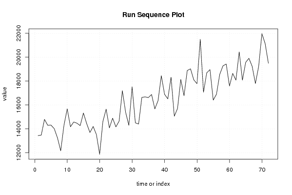
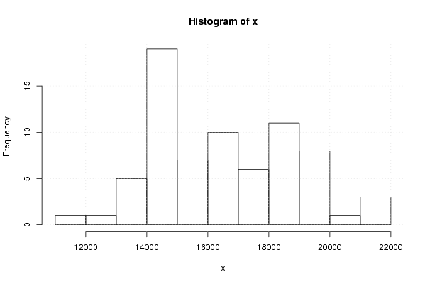
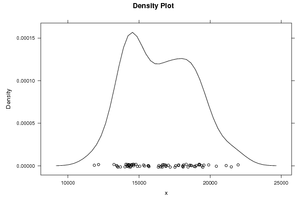
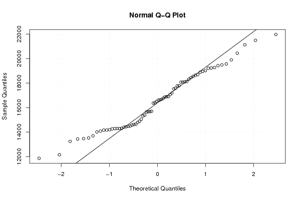
| Title produced by software | Univariate Explorative Data Analysis | ||||||||||||||||||||||||||||||||||||||||||||||||||||
| Date of computation | Wed, 17 Dec 2008 07:56:01 -0700 | ||||||||||||||||||||||||||||||||||||||||||||||||||||
| Cite this page as follows | Statistical Computations at FreeStatistics.org, Office for Research Development and Education, URL https://freestatistics.org/blog/index.php?v=date/2008/Dec/17/t122952584127xiu0i5e8h6ywj.htm/, Retrieved Sun, 19 May 2024 06:06:05 +0000 | ||||||||||||||||||||||||||||||||||||||||||||||||||||
| Statistical Computations at FreeStatistics.org, Office for Research Development and Education, URL https://freestatistics.org/blog/index.php?pk=34385, Retrieved Sun, 19 May 2024 06:06:05 +0000 | |||||||||||||||||||||||||||||||||||||||||||||||||||||
| QR Codes: | |||||||||||||||||||||||||||||||||||||||||||||||||||||
|
| |||||||||||||||||||||||||||||||||||||||||||||||||||||
| Original text written by user: | |||||||||||||||||||||||||||||||||||||||||||||||||||||
| IsPrivate? | No (this computation is public) | ||||||||||||||||||||||||||||||||||||||||||||||||||||
| User-defined keywords | |||||||||||||||||||||||||||||||||||||||||||||||||||||
| Estimated Impact | 172 | ||||||||||||||||||||||||||||||||||||||||||||||||||||
Tree of Dependent Computations | |||||||||||||||||||||||||||||||||||||||||||||||||||||
| Family? (F = Feedback message, R = changed R code, M = changed R Module, P = changed Parameters, D = changed Data) | |||||||||||||||||||||||||||||||||||||||||||||||||||||
| - [Mean versus Median] [Totale Invoer naa...] [2008-12-07 18:21:05] [299afd6311e4c20059ea2f05c8dd029d] - RM D [Variability] [Totale Invoer naa...] [2008-12-07 18:28:38] [299afd6311e4c20059ea2f05c8dd029d] - RMP [Stem-and-leaf Plot] [Totale Invoer naa...] [2008-12-07 18:32:41] [299afd6311e4c20059ea2f05c8dd029d] - RMPD [Quartiles] [Totale Invoer naa...] [2008-12-07 18:52:56] [299afd6311e4c20059ea2f05c8dd029d] - RM D [Harrell-Davis Quantiles] [Totale Invoer naa...] [2008-12-07 19:02:20] [299afd6311e4c20059ea2f05c8dd029d] - RM D [Pearson Correlation] [Totale Uitvoer vs...] [2008-12-07 19:10:32] [299afd6311e4c20059ea2f05c8dd029d] - RMPD [Univariate Explorative Data Analysis] [Totale invoer naa...] [2008-12-17 14:56:01] [5e2b1e7aa808f9f0d23fd35605d4968f] [Current] | |||||||||||||||||||||||||||||||||||||||||||||||||||||
| Feedback Forum | |||||||||||||||||||||||||||||||||||||||||||||||||||||
Post a new message | |||||||||||||||||||||||||||||||||||||||||||||||||||||
Dataset | |||||||||||||||||||||||||||||||||||||||||||||||||||||
| Dataseries X: | |||||||||||||||||||||||||||||||||||||||||||||||||||||
13429,9 13470,1 14785,8 14292 14308,8 14013 13240,9 12153,4 14289,7 15669,2 14169,5 14569,8 14469,1 14264,9 15320,9 14433,5 13691,5 14194,1 13519,2 11857,9 14616 15643,4 14077,2 14887,5 14159,9 14643 17192,5 15386,1 14287,1 17526,6 14497 14398,3 16629,6 16670,7 16614,8 16869,2 15663,9 16359,9 18447,7 16889 16505 18320,9 15052,1 15699,8 18135,3 16768,7 18883 19021 18101,9 17776,1 21489,9 17065,3 18690 18953,1 16398,9 16895,7 18553 19270 19422,1 17579,4 18637,3 18076,7 20438,6 18075,2 19563 19899,2 19227,5 17789,6 19220,8 21968,9 21131,5 19484,6 | |||||||||||||||||||||||||||||||||||||||||||||||||||||
Tables (Output of Computation) | |||||||||||||||||||||||||||||||||||||||||||||||||||||
| |||||||||||||||||||||||||||||||||||||||||||||||||||||
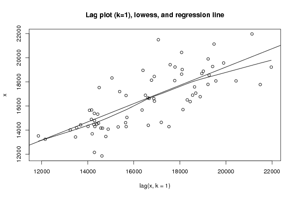
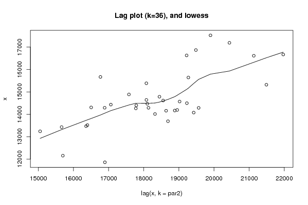
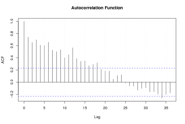
Figures (Output of Computation) | |||||||||||||||||||||||||||||||||||||||||||||||||||||
Input Parameters & R Code | |||||||||||||||||||||||||||||||||||||||||||||||||||||
| Parameters (Session): | |||||||||||||||||||||||||||||||||||||||||||||||||||||
| par1 = 0 ; par2 = 36 ; | |||||||||||||||||||||||||||||||||||||||||||||||||||||
| Parameters (R input): | |||||||||||||||||||||||||||||||||||||||||||||||||||||
| par1 = 0 ; par2 = 36 ; | |||||||||||||||||||||||||||||||||||||||||||||||||||||
| R code (references can be found in the software module): | |||||||||||||||||||||||||||||||||||||||||||||||||||||
par1 <- as.numeric(par1) | |||||||||||||||||||||||||||||||||||||||||||||||||||||