Repository of Reproducible Computations

Free Statistics

of Irreproducible Research!

Author's title

Author

*Unverified author*

R Software Module

rwasp_notchedbox1.wasp

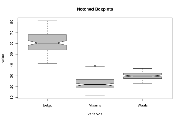
Title produced by software

Notched Boxplots

Date of computation

Wed, 17 Dec 2008 06:41:03 -0700

Cite this page as follows

Statistical Computations at FreeStatistics.org, Office for Research Development and Education, URL https://freestatistics.org/blog/index.php?v=date/2008/Dec/17/t1229521326e22lkf0b40fbm5p.htm/, Retrieved Sun, 19 May 2024 05:39:49 +0000

Statistical Computations at FreeStatistics.org, Office for Research Development and Education, URL https://freestatistics.org/blog/index.php?pk=34343, Retrieved Sun, 19 May 2024 05:39:49 +0000

QR Codes:

Paste this QR Code to cite your computation.

Original text written by user:

IsPrivate?

No (this computation is public)

User-defined keywords

marie_noyens@hotmail.com

Estimated Impact

159

Family? (F = Feedback message, R = changed R code, M = changed R Module, P = changed Parameters, D = changed Data)

-       [Notched Boxplots] [Paper notched box...] [2008-12-17 13:41:03] [bbcc60648878a43c4199b874b2670e4f] [Current]

Feedback Forum

Post a new message

Dataseries X:

Download CSV

Histogram

Boxplots

60.804	21.863	30.811
57.907	20.403	29.877
54.355	18.792	28.303
52.536	17.931	27.605
49.081	16.475	26.074
48.877	16.205	26.112
64.599	25.134	32.350
75.314	31.896	35.804
71.209	26.537	36.574
65.210	22.801	34.486
59.829	20.200	32.158
57.656	19.666	30.965
57.428	19.809	30.505
55.315	18.799	29.629
52.790	17.884	28.169
51.050	17.512	26.972
48.519	16.327	25.752
48.354	16.880	25.027
65.333	26.537	31.530
73.990	31.867	34.705
72.755	29.427	35.223
67.424	25.800	33.471
59.214	22.041	29.239
57.427	21.759	27.954
56.681	21.333	27.727
55.437	20.462	27.314
53.600	19.594	26.576
51.641	18.564	25.775
49.478	17.640	24.669
50.124	18.614	24.480
71.313	32.562	30.834
76.208	35.640	33.218
74.387	31.865	33.783
69.520	28.117	32.546
64.735	25.508	30.661
63.413	25.006	30.070
62.553	24.452	29.722
60.109	22.643	29.075
57.764	21.474	28.136
55.667	20.500	27.315
53.103	19.505	26.125
55.301	21.769	26.057
76.795	36.062	32.601
80.928	38.633	34.214
79.213	34.629	35.232
72.759	30.184	33.565
67.802	27.271	31.931
66.940	26.841	31.779
66.396	26.482	31.626
67.539	25.538	31.230
67.776	23.789	29.574
68.014	22.386	28.312
68.251	21.087	27.186
68.488	22.891	27.397
68.725	36.192	33.387
68.962	38.922	34.996
69.200	34.669	36.251
69.437	30.197	34.284
68.212	27.001	32.349
65.444	25.891	30.991
63.181	24.879	29.916
61.198	23.662	29.067
59.010	22.741	27.978
56.388	21.615	26.719
53.723	20.305	25.544
55.340	21.877	25.703
75.352	35.369	31.703
79.817	37.941	33.733
78.289	33.480	35.121
71.892	29.757	32.714
66.448	26.323	31.111
64.167	25.359	29.977
61.250	22.207	30.375
59.580	21.763	29.323
56.417	19.944	28.193
54.662	19.662	27.222
53.349	18.624	26.904
55.385	19.902	27.952
73.546	31.726	33.512
77.683	32.860	36.215
74.995	28.894	36.856
67.282	22.949	35.341
60.742	19.758	32.624
57.283	18.420	30.885
57.314	18.245	31.108
54.704	16.761	30.267
51.578	15.341	28.645
49.962	14.271	28.474
46.252	13.418	25.805
47.234	15.218	24.756
64.708	26.485	30.437
68.753	27.457	33.177
62.970	21.402	33.069
57.474	17.879	31.342
52.494	15.607	28.912
51.831	15.626	28.373
51.663	15.303	28.599
49.637	14.296	27.884
46.679	13.686	25.727
45.557	12.948	25.393
41.630	11.609	23.147
44.417	14.602	23.164
60.070	23.629	29.286
63.157	24.680	31.008

Summary of computational transaction
Raw Input	view raw input (R code)
Raw Output	view raw output of R engine
Computing time	1 seconds
R Server	'Gwilym Jenkins' @ 72.249.127.135

\begin{tabular}{lllllllll}
\hline
Summary of computational transaction \tabularnewline
Raw Input & view raw input (R code)  \tabularnewline
Raw Output & view raw output of R engine  \tabularnewline
Computing time & 1 seconds \tabularnewline
R Server & 'Gwilym Jenkins' @ 72.249.127.135 \tabularnewline
\hline
\end{tabular}
%Source: https://freestatistics.org/blog/index.php?pk=34343&T=0

[TABLE]
[ROW][C]Summary of computational transaction[/C][/ROW]
[ROW][C]Raw Input[/C][C]view raw input (R code) [/C][/ROW]
[ROW][C]Raw Output[/C][C]view raw output of R engine [/C][/ROW]
[ROW][C]Computing time[/C][C]1 seconds[/C][/ROW]
[ROW][C]R Server[/C][C]'Gwilym Jenkins' @ 72.249.127.135[/C][/ROW]
[/TABLE]
Source: https://freestatistics.org/blog/index.php?pk=34343&T=0

Globally Unique Identifier (entire table): ba.freestatistics.org/blog/index.php?pk=34343&T=0

As an alternative you can also use a QR Code:

The GUIDs for individual cells are displayed in the table below:

Summary of computational transaction
Raw Input	view raw input (R code)
Raw Output	view raw output of R engine
Computing time	1 seconds
R Server	'Gwilym Jenkins' @ 72.249.127.135

Boxplot statistics
Variable	lower whisker	lower hinge	median	upper hinge	upper whisker
Belgi�	41.63	54.039	60.4255	68.2315	80.928
Vlaams	11.609	18.619	21.959	26.689	38.633
Waals	23.147	27.501	29.9465	32.5735	36.856

\begin{tabular}{lllllllll}
\hline
Boxplot statistics \tabularnewline
Variable & lower whisker & lower hinge & median & upper hinge & upper whisker \tabularnewline
Belgi� & 41.63 & 54.039 & 60.4255 & 68.2315 & 80.928 \tabularnewline
Vlaams & 11.609 & 18.619 & 21.959 & 26.689 & 38.633 \tabularnewline
Waals & 23.147 & 27.501 & 29.9465 & 32.5735 & 36.856 \tabularnewline
\hline
\end{tabular}
%Source: https://freestatistics.org/blog/index.php?pk=34343&T=1

[TABLE]
[ROW][C]Boxplot statistics[/C][/ROW]
[ROW][C]Variable[/C][C]lower whisker[/C][C]lower hinge[/C][C]median[/C][C]upper hinge[/C][C]upper whisker[/C][/ROW]
[ROW][C]Belgi�[/C][C]41.63[/C][C]54.039[/C][C]60.4255[/C][C]68.2315[/C][C]80.928[/C][/ROW]
[ROW][C]Vlaams[/C][C]11.609[/C][C]18.619[/C][C]21.959[/C][C]26.689[/C][C]38.633[/C][/ROW]
[ROW][C]Waals[/C][C]23.147[/C][C]27.501[/C][C]29.9465[/C][C]32.5735[/C][C]36.856[/C][/ROW]
[/TABLE]
Source: https://freestatistics.org/blog/index.php?pk=34343&T=1

Globally Unique Identifier (entire table): ba.freestatistics.org/blog/index.php?pk=34343&T=1

As an alternative you can also use a QR Code:

The GUIDs for individual cells are displayed in the table below:

Boxplot statistics
Variable	lower whisker	lower hinge	median	upper hinge	upper whisker
Belgi�	41.63	54.039	60.4255	68.2315	80.928
Vlaams	11.609	18.619	21.959	26.689	38.633
Waals	23.147	27.501	29.9465	32.5735	36.856

Boxplot Notches
Variable	lower bound	median	upper bound
Belgi�	58.2266311841205	60.4255	62.6243688158795
Vlaams	20.7087008036535	21.959	23.2092991963465
Waals	29.1606087145641	29.9465	30.7323912854359

\begin{tabular}{lllllllll}
\hline
Boxplot Notches \tabularnewline
Variable & lower bound & median & upper bound \tabularnewline
Belgi� & 58.2266311841205 & 60.4255 & 62.6243688158795 \tabularnewline
Vlaams & 20.7087008036535 & 21.959 & 23.2092991963465 \tabularnewline
Waals & 29.1606087145641 & 29.9465 & 30.7323912854359 \tabularnewline
\hline
\end{tabular}
%Source: https://freestatistics.org/blog/index.php?pk=34343&T=2

[TABLE]
[ROW][C]Boxplot Notches[/C][/ROW]
[ROW][C]Variable[/C][C]lower bound[/C][C]median[/C][C]upper bound[/C][/ROW]
[ROW][C]Belgi�[/C][C]58.2266311841205[/C][C]60.4255[/C][C]62.6243688158795[/C][/ROW]
[ROW][C]Vlaams[/C][C]20.7087008036535[/C][C]21.959[/C][C]23.2092991963465[/C][/ROW]
[ROW][C]Waals[/C][C]29.1606087145641[/C][C]29.9465[/C][C]30.7323912854359[/C][/ROW]
[/TABLE]
Source: https://freestatistics.org/blog/index.php?pk=34343&T=2

Globally Unique Identifier (entire table): ba.freestatistics.org/blog/index.php?pk=34343&T=2

As an alternative you can also use a QR Code:

The GUIDs for individual cells are displayed in the table below:

Boxplot Notches
Variable	lower bound	median	upper bound
Belgi�	58.2266311841205	60.4255	62.6243688158795
Vlaams	20.7087008036535	21.959	23.2092991963465
Waals	29.1606087145641	29.9465	30.7323912854359

Figure 1

PNG link

Postscript link

PDF link

Parameters (Session):

par1 = grey ;

Parameters (R input):

par1 = grey ;

R code (references can be found in the software module):

z <- as.data.frame(t(y))
bitmap(file='test1.png')
(r<-boxplot(z ,xlab=xlab,ylab=ylab,main=main,notch=TRUE,col=par1))
dev.off()
load(file='createtable')
a<-table.start()
a<-table.row.start(a)
a<-table.element(a,hyperlink('overview.htm','Boxplot statistics','Boxplot overview'),6,TRUE)
a<-table.row.end(a)
a<-table.row.start(a)
a<-table.element(a,'Variable',1,TRUE)
a<-table.element(a,hyperlink('lower_whisker.htm','lower whisker','definition of lower whisker'),1,TRUE)
a<-table.element(a,hyperlink('lower_hinge.htm','lower hinge','definition of lower hinge'),1,TRUE)
a<-table.element(a,hyperlink('central_tendency.htm','median','definitions about measures of central tendency'),1,TRUE)
a<-table.element(a,hyperlink('upper_hinge.htm','upper hinge','definition of upper hinge'),1,TRUE)
a<-table.element(a,hyperlink('upper_whisker.htm','upper whisker','definition of upper whisker'),1,TRUE)
a<-table.row.end(a)
for (i in 1:length(y[,1]))
{
a<-table.row.start(a)
a<-table.element(a,dimnames(t(x))[[2]][i],1,TRUE)
for (j in 1:5)
{
a<-table.element(a,r$stats[j,i])
}
a<-table.row.end(a)
}
a<-table.end(a)
table.save(a,file='mytable.tab')
a<-table.start()
a<-table.row.start(a)
a<-table.element(a,'Boxplot Notches',4,TRUE)
a<-table.row.end(a)
a<-table.row.start(a)
a<-table.element(a,'Variable',1,TRUE)
a<-table.element(a,'lower bound',1,TRUE)
a<-table.element(a,'median',1,TRUE)
a<-table.element(a,'upper bound',1,TRUE)
a<-table.row.end(a)
for (i in 1:length(y[,1]))
{
a<-table.row.start(a)
a<-table.element(a,dimnames(t(x))[[2]][i],1,TRUE)
a<-table.element(a,r$conf[1,i])
a<-table.element(a,r$stats[3,i])
a<-table.element(a,r$conf[2,i])
a<-table.row.end(a)
}
a<-table.end(a)
table.save(a,file='mytable1.tab')

Free Statistics

Description of Statistical Computation

Tree of Dependent Computations

Dataset

Tables (Output of Computation)

Figures (Output of Computation)

Input Parameters & R Code