Repository of Reproducible Computations

Free Statistics

of Irreproducible Research!

Author's title

Author

*Unverified author*

R Software Module

rwasp_autocorrelation.wasp

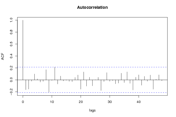
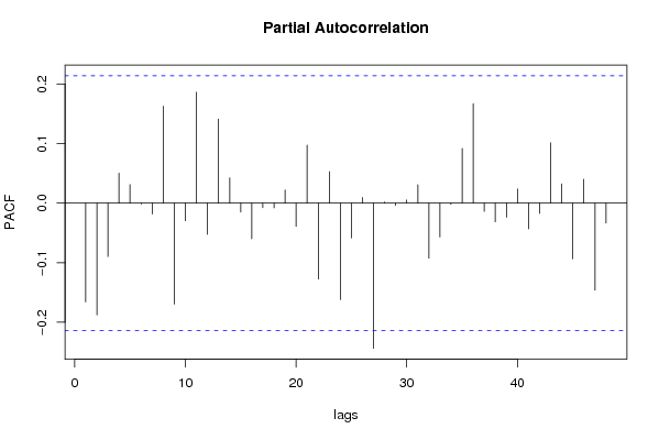
Title produced by software

(Partial) Autocorrelation Function

Date of computation

Wed, 17 Dec 2008 06:14:58 -0700

Cite this page as follows

Statistical Computations at FreeStatistics.org, Office for Research Development and Education, URL https://freestatistics.org/blog/index.php?v=date/2008/Dec/17/t1229519753pt8y5uotg2bmeuf.htm/, Retrieved Sun, 19 May 2024 04:28:25 +0000

Statistical Computations at FreeStatistics.org, Office for Research Development and Education, URL https://freestatistics.org/blog/index.php?pk=34330, Retrieved Sun, 19 May 2024 04:28:25 +0000

QR Codes:

Paste this QR Code to cite your computation.

Original text written by user:

IsPrivate?

No (this computation is public)

User-defined keywords

Estimated Impact

173

Family? (F = Feedback message, R = changed R code, M = changed R Module, P = changed Parameters, D = changed Data)

-     [] [] [1970-01-01 00:00:00] [2097edf1f094fab6879a8cb46df74ec2]
- RMPD  [(Partial) Autocorrelation Function] [] [2008-12-17 12:55:33] [2097edf1f094fab6879a8cb46df74ec2]
-   PD      [(Partial) Autocorrelation Function] [] [2008-12-17 13:14:58] [06e57c0cb32e2f613cf343ab1a0ac99f] [Current]
-   PD        [(Partial) Autocorrelation Function] [] [2008-12-17 13:23:48] [74be16979710d4c4e7c6647856088456] 
-   PD        [(Partial) Autocorrelation Function] [] [2008-12-17 13:25:37] [74be16979710d4c4e7c6647856088456] 

Feedback Forum

Post a new message

Dataseries X:

Download CSV

Histogram

Boxplots

1,63
1,63
1,62
1,62
1,61
1,6
1,6
1,6
1,59
1,59
1,58
1,58
1,58
1,58
1,58
1,58
1,56
1,56
1,55
1,55
1,55
1,54
1,54
1,53
1,53
1,53
1,53
1,52
1,52
1,52
1,52
1,51
1,51
1,51
1,5
1,49
1,49
1,49
1,48
1,47
1,47
1,47
1,46
1,46
1,45
1,45
1,44
1,43
1,43
1,43
1,42
1,41
1,4
1,4
1,4
1,4
1,39
1,38
1,38
1,38
1,37
1,37
1,37
1,37
1,37
1,37
1,37
1,36
1,36
1,36
1,35
1,34
1,34
1,34
1,34
1,34
1,34
1,34
1,33
1,33
1,33
1,32
1,32
1,32
1,32

Summary of computational transaction
Raw Input	view raw input (R code)
Raw Output	view raw output of R engine
Computing time	1 seconds
R Server	'George Udny Yule' @ 72.249.76.132

\begin{tabular}{lllllllll}
\hline
Summary of computational transaction \tabularnewline
Raw Input & view raw input (R code)  \tabularnewline
Raw Output & view raw output of R engine  \tabularnewline
Computing time & 1 seconds \tabularnewline
R Server & 'George Udny Yule' @ 72.249.76.132 \tabularnewline
\hline
\end{tabular}
%Source: https://freestatistics.org/blog/index.php?pk=34330&T=0

[TABLE]
[ROW][C]Summary of computational transaction[/C][/ROW]
[ROW][C]Raw Input[/C][C]view raw input (R code) [/C][/ROW]
[ROW][C]Raw Output[/C][C]view raw output of R engine [/C][/ROW]
[ROW][C]Computing time[/C][C]1 seconds[/C][/ROW]
[ROW][C]R Server[/C][C]'George Udny Yule' @ 72.249.76.132[/C][/ROW]
[/TABLE]
Source: https://freestatistics.org/blog/index.php?pk=34330&T=0

Globally Unique Identifier (entire table): ba.freestatistics.org/blog/index.php?pk=34330&T=0

As an alternative you can also use a QR Code:

The GUIDs for individual cells are displayed in the table below:

Summary of computational transaction
Raw Input	view raw input (R code)
Raw Output	view raw output of R engine
Computing time	1 seconds
R Server	'George Udny Yule' @ 72.249.76.132

Autocorrelation Function
Time lag k	ACF(k)	T-STAT	P-value
1	-0.165898	-1.5205	0.066073
2	-0.155097	-1.4215	0.079438
3	-0.022265	-0.2041	0.4194
4	0.09842	0.902	0.18481
5	0.016454	0.1508	0.440247
6	-0.036247	-0.3322	0.37028
7	-0.025446	-0.2332	0.408079
8	0.170887	1.5662	0.06053
9	-0.206496	-1.8926	0.03093
10	-0.010163	-0.0931	0.463006
11	0.215436	1.9745	0.025805
12	-0.06918	-0.634	0.263886
13	0.063652	0.5834	0.2806
14	-0.018314	-0.1679	0.433552
15	-0.007514	-0.0689	0.472631
16	-0.025979	-0.2381	0.406192
17	-0.032296	-0.296	0.383981
18	0.042005	0.385	0.350611
19	0.082071	0.7522	0.227018
20	-0.156162	-1.4312	0.078034
21	0.132938	1.2184	0.113243
22	-0.105296	-0.9651	0.168645
23	0.044654	0.4093	0.341694
24	-0.100812	-0.924	0.179076
25	0.002754	0.0252	0.48996
26	0.04282	0.3925	0.347858
27	-0.178295	-1.6341	0.05299
28	-0.028345	-0.2598	0.397831
29	0.121605	1.1145	0.134116
30	-0.023862	-0.2187	0.413707
31	-0.013062	-0.1197	0.452498
32	-0.065762	-0.6027	0.274159
33	-0.054962	-0.5037	0.307884
34	0.112106	1.0275	0.153575
35	-0.045509	-0.4171	0.338836
36	0.133707	1.2254	0.111917
37	-0.058143	-0.5329	0.297757
38	-0.169375	-1.5523	0.062169
39	0.044076	0.404	0.343634
40	0.084142	0.7712	0.221384
41	-0.090591	-0.8303	0.204368
42	0.059359	0.544	0.293928
43	-0.022607	-0.2072	0.41818
44	0.08096	0.742	0.230075
45	-0.157273	-1.4414	0.07659
46	0.009795	0.0898	0.464342
47	0.084096	0.7708	0.221508
48	-0.014988	-0.1374	0.445535

\begin{tabular}{lllllllll}
\hline
Autocorrelation Function \tabularnewline
Time lag k & ACF(k) & T-STAT & P-value \tabularnewline
1 & -0.165898 & -1.5205 & 0.066073 \tabularnewline
2 & -0.155097 & -1.4215 & 0.079438 \tabularnewline
3 & -0.022265 & -0.2041 & 0.4194 \tabularnewline
4 & 0.09842 & 0.902 & 0.18481 \tabularnewline
5 & 0.016454 & 0.1508 & 0.440247 \tabularnewline
6 & -0.036247 & -0.3322 & 0.37028 \tabularnewline
7 & -0.025446 & -0.2332 & 0.408079 \tabularnewline
8 & 0.170887 & 1.5662 & 0.06053 \tabularnewline
9 & -0.206496 & -1.8926 & 0.03093 \tabularnewline
10 & -0.010163 & -0.0931 & 0.463006 \tabularnewline
11 & 0.215436 & 1.9745 & 0.025805 \tabularnewline
12 & -0.06918 & -0.634 & 0.263886 \tabularnewline
13 & 0.063652 & 0.5834 & 0.2806 \tabularnewline
14 & -0.018314 & -0.1679 & 0.433552 \tabularnewline
15 & -0.007514 & -0.0689 & 0.472631 \tabularnewline
16 & -0.025979 & -0.2381 & 0.406192 \tabularnewline
17 & -0.032296 & -0.296 & 0.383981 \tabularnewline
18 & 0.042005 & 0.385 & 0.350611 \tabularnewline
19 & 0.082071 & 0.7522 & 0.227018 \tabularnewline
20 & -0.156162 & -1.4312 & 0.078034 \tabularnewline
21 & 0.132938 & 1.2184 & 0.113243 \tabularnewline
22 & -0.105296 & -0.9651 & 0.168645 \tabularnewline
23 & 0.044654 & 0.4093 & 0.341694 \tabularnewline
24 & -0.100812 & -0.924 & 0.179076 \tabularnewline
25 & 0.002754 & 0.0252 & 0.48996 \tabularnewline
26 & 0.04282 & 0.3925 & 0.347858 \tabularnewline
27 & -0.178295 & -1.6341 & 0.05299 \tabularnewline
28 & -0.028345 & -0.2598 & 0.397831 \tabularnewline
29 & 0.121605 & 1.1145 & 0.134116 \tabularnewline
30 & -0.023862 & -0.2187 & 0.413707 \tabularnewline
31 & -0.013062 & -0.1197 & 0.452498 \tabularnewline
32 & -0.065762 & -0.6027 & 0.274159 \tabularnewline
33 & -0.054962 & -0.5037 & 0.307884 \tabularnewline
34 & 0.112106 & 1.0275 & 0.153575 \tabularnewline
35 & -0.045509 & -0.4171 & 0.338836 \tabularnewline
36 & 0.133707 & 1.2254 & 0.111917 \tabularnewline
37 & -0.058143 & -0.5329 & 0.297757 \tabularnewline
38 & -0.169375 & -1.5523 & 0.062169 \tabularnewline
39 & 0.044076 & 0.404 & 0.343634 \tabularnewline
40 & 0.084142 & 0.7712 & 0.221384 \tabularnewline
41 & -0.090591 & -0.8303 & 0.204368 \tabularnewline
42 & 0.059359 & 0.544 & 0.293928 \tabularnewline
43 & -0.022607 & -0.2072 & 0.41818 \tabularnewline
44 & 0.08096 & 0.742 & 0.230075 \tabularnewline
45 & -0.157273 & -1.4414 & 0.07659 \tabularnewline
46 & 0.009795 & 0.0898 & 0.464342 \tabularnewline
47 & 0.084096 & 0.7708 & 0.221508 \tabularnewline
48 & -0.014988 & -0.1374 & 0.445535 \tabularnewline
\hline
\end{tabular}
%Source: https://freestatistics.org/blog/index.php?pk=34330&T=1

[TABLE]
[ROW][C]Autocorrelation Function[/C][/ROW]
[ROW][C]Time lag k[/C][C]ACF(k)[/C][C]T-STAT[/C][C]P-value[/C][/ROW]
[ROW][C]1[/C][C]-0.165898[/C][C]-1.5205[/C][C]0.066073[/C][/ROW]
[ROW][C]2[/C][C]-0.155097[/C][C]-1.4215[/C][C]0.079438[/C][/ROW]
[ROW][C]3[/C][C]-0.022265[/C][C]-0.2041[/C][C]0.4194[/C][/ROW]
[ROW][C]4[/C][C]0.09842[/C][C]0.902[/C][C]0.18481[/C][/ROW]
[ROW][C]5[/C][C]0.016454[/C][C]0.1508[/C][C]0.440247[/C][/ROW]
[ROW][C]6[/C][C]-0.036247[/C][C]-0.3322[/C][C]0.37028[/C][/ROW]
[ROW][C]7[/C][C]-0.025446[/C][C]-0.2332[/C][C]0.408079[/C][/ROW]
[ROW][C]8[/C][C]0.170887[/C][C]1.5662[/C][C]0.06053[/C][/ROW]
[ROW][C]9[/C][C]-0.206496[/C][C]-1.8926[/C][C]0.03093[/C][/ROW]
[ROW][C]10[/C][C]-0.010163[/C][C]-0.0931[/C][C]0.463006[/C][/ROW]
[ROW][C]11[/C][C]0.215436[/C][C]1.9745[/C][C]0.025805[/C][/ROW]
[ROW][C]12[/C][C]-0.06918[/C][C]-0.634[/C][C]0.263886[/C][/ROW]
[ROW][C]13[/C][C]0.063652[/C][C]0.5834[/C][C]0.2806[/C][/ROW]
[ROW][C]14[/C][C]-0.018314[/C][C]-0.1679[/C][C]0.433552[/C][/ROW]
[ROW][C]15[/C][C]-0.007514[/C][C]-0.0689[/C][C]0.472631[/C][/ROW]
[ROW][C]16[/C][C]-0.025979[/C][C]-0.2381[/C][C]0.406192[/C][/ROW]
[ROW][C]17[/C][C]-0.032296[/C][C]-0.296[/C][C]0.383981[/C][/ROW]
[ROW][C]18[/C][C]0.042005[/C][C]0.385[/C][C]0.350611[/C][/ROW]
[ROW][C]19[/C][C]0.082071[/C][C]0.7522[/C][C]0.227018[/C][/ROW]
[ROW][C]20[/C][C]-0.156162[/C][C]-1.4312[/C][C]0.078034[/C][/ROW]
[ROW][C]21[/C][C]0.132938[/C][C]1.2184[/C][C]0.113243[/C][/ROW]
[ROW][C]22[/C][C]-0.105296[/C][C]-0.9651[/C][C]0.168645[/C][/ROW]
[ROW][C]23[/C][C]0.044654[/C][C]0.4093[/C][C]0.341694[/C][/ROW]
[ROW][C]24[/C][C]-0.100812[/C][C]-0.924[/C][C]0.179076[/C][/ROW]
[ROW][C]25[/C][C]0.002754[/C][C]0.0252[/C][C]0.48996[/C][/ROW]
[ROW][C]26[/C][C]0.04282[/C][C]0.3925[/C][C]0.347858[/C][/ROW]
[ROW][C]27[/C][C]-0.178295[/C][C]-1.6341[/C][C]0.05299[/C][/ROW]
[ROW][C]28[/C][C]-0.028345[/C][C]-0.2598[/C][C]0.397831[/C][/ROW]
[ROW][C]29[/C][C]0.121605[/C][C]1.1145[/C][C]0.134116[/C][/ROW]
[ROW][C]30[/C][C]-0.023862[/C][C]-0.2187[/C][C]0.413707[/C][/ROW]
[ROW][C]31[/C][C]-0.013062[/C][C]-0.1197[/C][C]0.452498[/C][/ROW]
[ROW][C]32[/C][C]-0.065762[/C][C]-0.6027[/C][C]0.274159[/C][/ROW]
[ROW][C]33[/C][C]-0.054962[/C][C]-0.5037[/C][C]0.307884[/C][/ROW]
[ROW][C]34[/C][C]0.112106[/C][C]1.0275[/C][C]0.153575[/C][/ROW]
[ROW][C]35[/C][C]-0.045509[/C][C]-0.4171[/C][C]0.338836[/C][/ROW]
[ROW][C]36[/C][C]0.133707[/C][C]1.2254[/C][C]0.111917[/C][/ROW]
[ROW][C]37[/C][C]-0.058143[/C][C]-0.5329[/C][C]0.297757[/C][/ROW]
[ROW][C]38[/C][C]-0.169375[/C][C]-1.5523[/C][C]0.062169[/C][/ROW]
[ROW][C]39[/C][C]0.044076[/C][C]0.404[/C][C]0.343634[/C][/ROW]
[ROW][C]40[/C][C]0.084142[/C][C]0.7712[/C][C]0.221384[/C][/ROW]
[ROW][C]41[/C][C]-0.090591[/C][C]-0.8303[/C][C]0.204368[/C][/ROW]
[ROW][C]42[/C][C]0.059359[/C][C]0.544[/C][C]0.293928[/C][/ROW]
[ROW][C]43[/C][C]-0.022607[/C][C]-0.2072[/C][C]0.41818[/C][/ROW]
[ROW][C]44[/C][C]0.08096[/C][C]0.742[/C][C]0.230075[/C][/ROW]
[ROW][C]45[/C][C]-0.157273[/C][C]-1.4414[/C][C]0.07659[/C][/ROW]
[ROW][C]46[/C][C]0.009795[/C][C]0.0898[/C][C]0.464342[/C][/ROW]
[ROW][C]47[/C][C]0.084096[/C][C]0.7708[/C][C]0.221508[/C][/ROW]
[ROW][C]48[/C][C]-0.014988[/C][C]-0.1374[/C][C]0.445535[/C][/ROW]
[/TABLE]
Source: https://freestatistics.org/blog/index.php?pk=34330&T=1

Globally Unique Identifier (entire table): ba.freestatistics.org/blog/index.php?pk=34330&T=1

As an alternative you can also use a QR Code:

The GUIDs for individual cells are displayed in the table below:

Autocorrelation Function
Time lag k	ACF(k)	T-STAT	P-value
1	-0.165898	-1.5205	0.066073
2	-0.155097	-1.4215	0.079438
3	-0.022265	-0.2041	0.4194
4	0.09842	0.902	0.18481
5	0.016454	0.1508	0.440247
6	-0.036247	-0.3322	0.37028
7	-0.025446	-0.2332	0.408079
8	0.170887	1.5662	0.06053
9	-0.206496	-1.8926	0.03093
10	-0.010163	-0.0931	0.463006
11	0.215436	1.9745	0.025805
12	-0.06918	-0.634	0.263886
13	0.063652	0.5834	0.2806
14	-0.018314	-0.1679	0.433552
15	-0.007514	-0.0689	0.472631
16	-0.025979	-0.2381	0.406192
17	-0.032296	-0.296	0.383981
18	0.042005	0.385	0.350611
19	0.082071	0.7522	0.227018
20	-0.156162	-1.4312	0.078034
21	0.132938	1.2184	0.113243
22	-0.105296	-0.9651	0.168645
23	0.044654	0.4093	0.341694
24	-0.100812	-0.924	0.179076
25	0.002754	0.0252	0.48996
26	0.04282	0.3925	0.347858
27	-0.178295	-1.6341	0.05299
28	-0.028345	-0.2598	0.397831
29	0.121605	1.1145	0.134116
30	-0.023862	-0.2187	0.413707
31	-0.013062	-0.1197	0.452498
32	-0.065762	-0.6027	0.274159
33	-0.054962	-0.5037	0.307884
34	0.112106	1.0275	0.153575
35	-0.045509	-0.4171	0.338836
36	0.133707	1.2254	0.111917
37	-0.058143	-0.5329	0.297757
38	-0.169375	-1.5523	0.062169
39	0.044076	0.404	0.343634
40	0.084142	0.7712	0.221384
41	-0.090591	-0.8303	0.204368
42	0.059359	0.544	0.293928
43	-0.022607	-0.2072	0.41818
44	0.08096	0.742	0.230075
45	-0.157273	-1.4414	0.07659
46	0.009795	0.0898	0.464342
47	0.084096	0.7708	0.221508
48	-0.014988	-0.1374	0.445535

Partial Autocorrelation Function
Time lag k	PACF(k)	T-STAT	P-value
1	-0.165898	-1.5205	0.066073
2	-0.187787	-1.7211	0.044457
3	-0.089514	-0.8204	0.207153
4	0.050445	0.4623	0.322519
5	0.031103	0.2851	0.388149
6	-0.001556	-0.0143	0.494326
7	-0.018313	-0.1678	0.433556
8	0.162904	1.493	0.069587
9	-0.169637	-1.5547	0.061883
10	-0.029507	-0.2704	0.393743
11	0.186305	1.7075	0.04571
12	-0.052368	-0.48	0.316251
13	0.141317	1.2952	0.099401
14	0.04241	0.3887	0.349242
15	-0.015076	-0.1382	0.445216
16	-0.059763	-0.5477	0.292661
17	-0.00771	-0.0707	0.471919
18	-0.007931	-0.0727	0.471113
19	0.022192	0.2034	0.419659
20	-0.038946	-0.357	0.361012
21	0.097554	0.8941	0.186913
22	-0.127616	-1.1696	0.122731
23	0.05291	0.4849	0.314494
24	-0.162204	-1.4866	0.070429
25	-0.058339	-0.5347	0.297138
26	0.009519	0.0872	0.465341
27	-0.243843	-2.2349	0.014041
28	0.001879	0.0172	0.49315
29	-0.003843	-0.0352	0.485993
30	0.005332	0.0489	0.480571
31	0.030942	0.2836	0.388711
32	-0.092398	-0.8468	0.199745
33	-0.056815	-0.5207	0.301966
34	-0.002113	-0.0194	0.492297
35	0.091945	0.8427	0.200897
36	0.166957	1.5302	0.064864
37	-0.013878	-0.1272	0.449546
38	-0.031459	-0.2883	0.386905
39	-0.023749	-0.2177	0.414111
40	0.023881	0.2189	0.413639
41	-0.043304	-0.3969	0.346227
42	-0.017263	-0.1582	0.437332
43	0.101343	0.9288	0.177822
44	0.032257	0.2956	0.384118
45	-0.093592	-0.8578	0.196726
46	0.040157	0.368	0.356883
47	-0.146227	-1.3402	0.091898
48	-0.033312	-0.3053	0.380441

\begin{tabular}{lllllllll}
\hline
Partial Autocorrelation Function \tabularnewline
Time lag k & PACF(k) & T-STAT & P-value \tabularnewline
1 & -0.165898 & -1.5205 & 0.066073 \tabularnewline
2 & -0.187787 & -1.7211 & 0.044457 \tabularnewline
3 & -0.089514 & -0.8204 & 0.207153 \tabularnewline
4 & 0.050445 & 0.4623 & 0.322519 \tabularnewline
5 & 0.031103 & 0.2851 & 0.388149 \tabularnewline
6 & -0.001556 & -0.0143 & 0.494326 \tabularnewline
7 & -0.018313 & -0.1678 & 0.433556 \tabularnewline
8 & 0.162904 & 1.493 & 0.069587 \tabularnewline
9 & -0.169637 & -1.5547 & 0.061883 \tabularnewline
10 & -0.029507 & -0.2704 & 0.393743 \tabularnewline
11 & 0.186305 & 1.7075 & 0.04571 \tabularnewline
12 & -0.052368 & -0.48 & 0.316251 \tabularnewline
13 & 0.141317 & 1.2952 & 0.099401 \tabularnewline
14 & 0.04241 & 0.3887 & 0.349242 \tabularnewline
15 & -0.015076 & -0.1382 & 0.445216 \tabularnewline
16 & -0.059763 & -0.5477 & 0.292661 \tabularnewline
17 & -0.00771 & -0.0707 & 0.471919 \tabularnewline
18 & -0.007931 & -0.0727 & 0.471113 \tabularnewline
19 & 0.022192 & 0.2034 & 0.419659 \tabularnewline
20 & -0.038946 & -0.357 & 0.361012 \tabularnewline
21 & 0.097554 & 0.8941 & 0.186913 \tabularnewline
22 & -0.127616 & -1.1696 & 0.122731 \tabularnewline
23 & 0.05291 & 0.4849 & 0.314494 \tabularnewline
24 & -0.162204 & -1.4866 & 0.070429 \tabularnewline
25 & -0.058339 & -0.5347 & 0.297138 \tabularnewline
26 & 0.009519 & 0.0872 & 0.465341 \tabularnewline
27 & -0.243843 & -2.2349 & 0.014041 \tabularnewline
28 & 0.001879 & 0.0172 & 0.49315 \tabularnewline
29 & -0.003843 & -0.0352 & 0.485993 \tabularnewline
30 & 0.005332 & 0.0489 & 0.480571 \tabularnewline
31 & 0.030942 & 0.2836 & 0.388711 \tabularnewline
32 & -0.092398 & -0.8468 & 0.199745 \tabularnewline
33 & -0.056815 & -0.5207 & 0.301966 \tabularnewline
34 & -0.002113 & -0.0194 & 0.492297 \tabularnewline
35 & 0.091945 & 0.8427 & 0.200897 \tabularnewline
36 & 0.166957 & 1.5302 & 0.064864 \tabularnewline
37 & -0.013878 & -0.1272 & 0.449546 \tabularnewline
38 & -0.031459 & -0.2883 & 0.386905 \tabularnewline
39 & -0.023749 & -0.2177 & 0.414111 \tabularnewline
40 & 0.023881 & 0.2189 & 0.413639 \tabularnewline
41 & -0.043304 & -0.3969 & 0.346227 \tabularnewline
42 & -0.017263 & -0.1582 & 0.437332 \tabularnewline
43 & 0.101343 & 0.9288 & 0.177822 \tabularnewline
44 & 0.032257 & 0.2956 & 0.384118 \tabularnewline
45 & -0.093592 & -0.8578 & 0.196726 \tabularnewline
46 & 0.040157 & 0.368 & 0.356883 \tabularnewline
47 & -0.146227 & -1.3402 & 0.091898 \tabularnewline
48 & -0.033312 & -0.3053 & 0.380441 \tabularnewline
\hline
\end{tabular}
%Source: https://freestatistics.org/blog/index.php?pk=34330&T=2

[TABLE]
[ROW][C]Partial Autocorrelation Function[/C][/ROW]
[ROW][C]Time lag k[/C][C]PACF(k)[/C][C]T-STAT[/C][C]P-value[/C][/ROW]
[ROW][C]1[/C][C]-0.165898[/C][C]-1.5205[/C][C]0.066073[/C][/ROW]
[ROW][C]2[/C][C]-0.187787[/C][C]-1.7211[/C][C]0.044457[/C][/ROW]
[ROW][C]3[/C][C]-0.089514[/C][C]-0.8204[/C][C]0.207153[/C][/ROW]
[ROW][C]4[/C][C]0.050445[/C][C]0.4623[/C][C]0.322519[/C][/ROW]
[ROW][C]5[/C][C]0.031103[/C][C]0.2851[/C][C]0.388149[/C][/ROW]
[ROW][C]6[/C][C]-0.001556[/C][C]-0.0143[/C][C]0.494326[/C][/ROW]
[ROW][C]7[/C][C]-0.018313[/C][C]-0.1678[/C][C]0.433556[/C][/ROW]
[ROW][C]8[/C][C]0.162904[/C][C]1.493[/C][C]0.069587[/C][/ROW]
[ROW][C]9[/C][C]-0.169637[/C][C]-1.5547[/C][C]0.061883[/C][/ROW]
[ROW][C]10[/C][C]-0.029507[/C][C]-0.2704[/C][C]0.393743[/C][/ROW]
[ROW][C]11[/C][C]0.186305[/C][C]1.7075[/C][C]0.04571[/C][/ROW]
[ROW][C]12[/C][C]-0.052368[/C][C]-0.48[/C][C]0.316251[/C][/ROW]
[ROW][C]13[/C][C]0.141317[/C][C]1.2952[/C][C]0.099401[/C][/ROW]
[ROW][C]14[/C][C]0.04241[/C][C]0.3887[/C][C]0.349242[/C][/ROW]
[ROW][C]15[/C][C]-0.015076[/C][C]-0.1382[/C][C]0.445216[/C][/ROW]
[ROW][C]16[/C][C]-0.059763[/C][C]-0.5477[/C][C]0.292661[/C][/ROW]
[ROW][C]17[/C][C]-0.00771[/C][C]-0.0707[/C][C]0.471919[/C][/ROW]
[ROW][C]18[/C][C]-0.007931[/C][C]-0.0727[/C][C]0.471113[/C][/ROW]
[ROW][C]19[/C][C]0.022192[/C][C]0.2034[/C][C]0.419659[/C][/ROW]
[ROW][C]20[/C][C]-0.038946[/C][C]-0.357[/C][C]0.361012[/C][/ROW]
[ROW][C]21[/C][C]0.097554[/C][C]0.8941[/C][C]0.186913[/C][/ROW]
[ROW][C]22[/C][C]-0.127616[/C][C]-1.1696[/C][C]0.122731[/C][/ROW]
[ROW][C]23[/C][C]0.05291[/C][C]0.4849[/C][C]0.314494[/C][/ROW]
[ROW][C]24[/C][C]-0.162204[/C][C]-1.4866[/C][C]0.070429[/C][/ROW]
[ROW][C]25[/C][C]-0.058339[/C][C]-0.5347[/C][C]0.297138[/C][/ROW]
[ROW][C]26[/C][C]0.009519[/C][C]0.0872[/C][C]0.465341[/C][/ROW]
[ROW][C]27[/C][C]-0.243843[/C][C]-2.2349[/C][C]0.014041[/C][/ROW]
[ROW][C]28[/C][C]0.001879[/C][C]0.0172[/C][C]0.49315[/C][/ROW]
[ROW][C]29[/C][C]-0.003843[/C][C]-0.0352[/C][C]0.485993[/C][/ROW]
[ROW][C]30[/C][C]0.005332[/C][C]0.0489[/C][C]0.480571[/C][/ROW]
[ROW][C]31[/C][C]0.030942[/C][C]0.2836[/C][C]0.388711[/C][/ROW]
[ROW][C]32[/C][C]-0.092398[/C][C]-0.8468[/C][C]0.199745[/C][/ROW]
[ROW][C]33[/C][C]-0.056815[/C][C]-0.5207[/C][C]0.301966[/C][/ROW]
[ROW][C]34[/C][C]-0.002113[/C][C]-0.0194[/C][C]0.492297[/C][/ROW]
[ROW][C]35[/C][C]0.091945[/C][C]0.8427[/C][C]0.200897[/C][/ROW]
[ROW][C]36[/C][C]0.166957[/C][C]1.5302[/C][C]0.064864[/C][/ROW]
[ROW][C]37[/C][C]-0.013878[/C][C]-0.1272[/C][C]0.449546[/C][/ROW]
[ROW][C]38[/C][C]-0.031459[/C][C]-0.2883[/C][C]0.386905[/C][/ROW]
[ROW][C]39[/C][C]-0.023749[/C][C]-0.2177[/C][C]0.414111[/C][/ROW]
[ROW][C]40[/C][C]0.023881[/C][C]0.2189[/C][C]0.413639[/C][/ROW]
[ROW][C]41[/C][C]-0.043304[/C][C]-0.3969[/C][C]0.346227[/C][/ROW]
[ROW][C]42[/C][C]-0.017263[/C][C]-0.1582[/C][C]0.437332[/C][/ROW]
[ROW][C]43[/C][C]0.101343[/C][C]0.9288[/C][C]0.177822[/C][/ROW]
[ROW][C]44[/C][C]0.032257[/C][C]0.2956[/C][C]0.384118[/C][/ROW]
[ROW][C]45[/C][C]-0.093592[/C][C]-0.8578[/C][C]0.196726[/C][/ROW]
[ROW][C]46[/C][C]0.040157[/C][C]0.368[/C][C]0.356883[/C][/ROW]
[ROW][C]47[/C][C]-0.146227[/C][C]-1.3402[/C][C]0.091898[/C][/ROW]
[ROW][C]48[/C][C]-0.033312[/C][C]-0.3053[/C][C]0.380441[/C][/ROW]
[/TABLE]
Source: https://freestatistics.org/blog/index.php?pk=34330&T=2

Globally Unique Identifier (entire table): ba.freestatistics.org/blog/index.php?pk=34330&T=2

As an alternative you can also use a QR Code:

The GUIDs for individual cells are displayed in the table below:

Partial Autocorrelation Function
Time lag k	PACF(k)	T-STAT	P-value
1	-0.165898	-1.5205	0.066073
2	-0.187787	-1.7211	0.044457
3	-0.089514	-0.8204	0.207153
4	0.050445	0.4623	0.322519
5	0.031103	0.2851	0.388149
6	-0.001556	-0.0143	0.494326
7	-0.018313	-0.1678	0.433556
8	0.162904	1.493	0.069587
9	-0.169637	-1.5547	0.061883
10	-0.029507	-0.2704	0.393743
11	0.186305	1.7075	0.04571
12	-0.052368	-0.48	0.316251
13	0.141317	1.2952	0.099401
14	0.04241	0.3887	0.349242
15	-0.015076	-0.1382	0.445216
16	-0.059763	-0.5477	0.292661
17	-0.00771	-0.0707	0.471919
18	-0.007931	-0.0727	0.471113
19	0.022192	0.2034	0.419659
20	-0.038946	-0.357	0.361012
21	0.097554	0.8941	0.186913
22	-0.127616	-1.1696	0.122731
23	0.05291	0.4849	0.314494
24	-0.162204	-1.4866	0.070429
25	-0.058339	-0.5347	0.297138
26	0.009519	0.0872	0.465341
27	-0.243843	-2.2349	0.014041
28	0.001879	0.0172	0.49315
29	-0.003843	-0.0352	0.485993
30	0.005332	0.0489	0.480571
31	0.030942	0.2836	0.388711
32	-0.092398	-0.8468	0.199745
33	-0.056815	-0.5207	0.301966
34	-0.002113	-0.0194	0.492297
35	0.091945	0.8427	0.200897
36	0.166957	1.5302	0.064864
37	-0.013878	-0.1272	0.449546
38	-0.031459	-0.2883	0.386905
39	-0.023749	-0.2177	0.414111
40	0.023881	0.2189	0.413639
41	-0.043304	-0.3969	0.346227
42	-0.017263	-0.1582	0.437332
43	0.101343	0.9288	0.177822
44	0.032257	0.2956	0.384118
45	-0.093592	-0.8578	0.196726
46	0.040157	0.368	0.356883
47	-0.146227	-1.3402	0.091898
48	-0.033312	-0.3053	0.380441

Figure 1

PNG link

Postscript link

PDF link

Figure 2

PNG link

Postscript link

PDF link

Parameters (Session):

par1 = 48 ; par2 = 1 ; par3 = 1 ; par4 = 0 ; par5 = 12 ;

Parameters (R input):

par1 = 48 ; par2 = 1 ; par3 = 1 ; par4 = 0 ; par5 = 12 ;

R code (references can be found in the software module):

if (par1 == 'Default') {
par1 = 10*log10(length(x))
} else {
par1 <- as.numeric(par1)
}
par2 <- as.numeric(par2)
par3 <- as.numeric(par3)
par4 <- as.numeric(par4)
par5 <- as.numeric(par5)
if (par2 == 0) {
x <- log(x)
} else {
x <- (x ^ par2 - 1) / par2
}
if (par3 > 0) x <- diff(x,lag=1,difference=par3)
if (par4 > 0) x <- diff(x,lag=par5,difference=par4)
bitmap(file='pic1.png')
racf <- acf(x,par1,main='Autocorrelation',xlab='lags',ylab='ACF')
dev.off()
bitmap(file='pic2.png')
rpacf <- pacf(x,par1,main='Partial Autocorrelation',xlab='lags',ylab='PACF')
dev.off()
(myacf <- c(racf$acf))
(mypacf <- c(rpacf$acf))
lengthx <- length(x)
sqrtn <- sqrt(lengthx)
load(file='createtable')
a<-table.start()
a<-table.row.start(a)
a<-table.element(a,'Autocorrelation Function',4,TRUE)
a<-table.row.end(a)
a<-table.row.start(a)
a<-table.element(a,'Time lag k',header=TRUE)
a<-table.element(a,hyperlink('basics.htm','ACF(k)','click here for more information about the Autocorrelation Function'),header=TRUE)
a<-table.element(a,'T-STAT',header=TRUE)
a<-table.element(a,'P-value',header=TRUE)
a<-table.row.end(a)
for (i in 2:(par1+1)) {
a<-table.row.start(a)
a<-table.element(a,i-1,header=TRUE)
a<-table.element(a,round(myacf[i],6))
mytstat <- myacf[i]*sqrtn
a<-table.element(a,round(mytstat,4))
a<-table.element(a,round(1-pt(abs(mytstat),lengthx),6))
a<-table.row.end(a)
}
a<-table.end(a)
table.save(a,file='mytable.tab')
a<-table.start()
a<-table.row.start(a)
a<-table.element(a,'Partial Autocorrelation Function',4,TRUE)
a<-table.row.end(a)
a<-table.row.start(a)
a<-table.element(a,'Time lag k',header=TRUE)
a<-table.element(a,hyperlink('basics.htm','PACF(k)','click here for more information about the Partial Autocorrelation Function'),header=TRUE)
a<-table.element(a,'T-STAT',header=TRUE)
a<-table.element(a,'P-value',header=TRUE)
a<-table.row.end(a)
for (i in 1:par1) {
a<-table.row.start(a)
a<-table.element(a,i,header=TRUE)
a<-table.element(a,round(mypacf[i],6))
mytstat <- mypacf[i]*sqrtn
a<-table.element(a,round(mytstat,4))
a<-table.element(a,round(1-pt(abs(mytstat),lengthx),6))
a<-table.row.end(a)
}
a<-table.end(a)
table.save(a,file='mytable1.tab')

Free Statistics

Description of Statistical Computation

Tree of Dependent Computations

Dataset

Tables (Output of Computation)

Figures (Output of Computation)

Input Parameters & R Code