Free Statistics
of Irreproducible Research!
Description of Statistical Computation | |||||||||||||||||||||
|---|---|---|---|---|---|---|---|---|---|---|---|---|---|---|---|---|---|---|---|---|---|
| Author's title | |||||||||||||||||||||
| Author | *The author of this computation has been verified* | ||||||||||||||||||||
| R Software Module | rwasp_meanplot.wasp | ||||||||||||||||||||
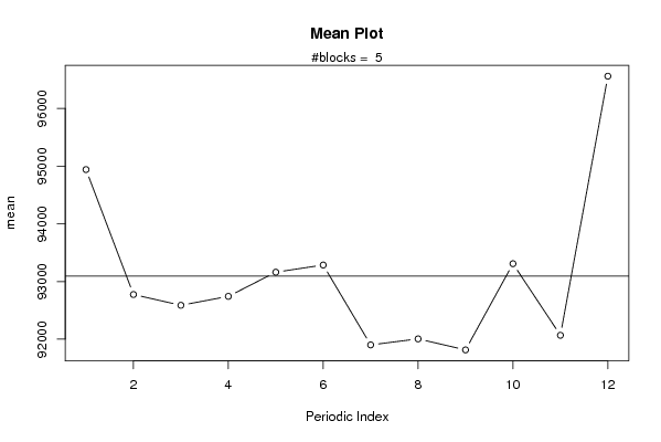
| Title produced by software | Mean Plot | ||||||||||||||||||||
| Date of computation | Sat, 13 Dec 2008 14:33:10 -0700 | ||||||||||||||||||||
| Cite this page as follows | Statistical Computations at FreeStatistics.org, Office for Research Development and Education, URL https://freestatistics.org/blog/index.php?v=date/2008/Dec/13/t1229204072lruseei10tf9a77.htm/, Retrieved Sun, 19 May 2024 05:36:18 +0000 | ||||||||||||||||||||
| Statistical Computations at FreeStatistics.org, Office for Research Development and Education, URL https://freestatistics.org/blog/index.php?pk=33223, Retrieved Sun, 19 May 2024 05:36:18 +0000 | |||||||||||||||||||||
| QR Codes: | |||||||||||||||||||||
|
| |||||||||||||||||||||
| Original text written by user: | |||||||||||||||||||||
| IsPrivate? | No (this computation is public) | ||||||||||||||||||||
| User-defined keywords | |||||||||||||||||||||
| Estimated Impact | 175 | ||||||||||||||||||||
Tree of Dependent Computations | |||||||||||||||||||||
| Family? (F = Feedback message, R = changed R code, M = changed R Module, P = changed Parameters, D = changed Data) | |||||||||||||||||||||
| - [Mean Plot] [Mean plot vervaar...] [2007-11-09 12:25:12] [74be16979710d4c4e7c6647856088456] - R D [Mean Plot] [Mean plot Vlaams ...] [2008-12-13 21:24:44] [005293453b571dbccb80b45226e44173] - D [Mean Plot] [Mean plot waals g...] [2008-12-13 21:27:39] [005293453b571dbccb80b45226e44173] - D [Mean Plot] [mean plot brussel...] [2008-12-13 21:33:10] [b0654df83a8a0e1de3ceb7bf60f0d58f] [Current] - D [Mean Plot] [mean plot Belgi�] [2008-12-13 21:36:14] [005293453b571dbccb80b45226e44173] | |||||||||||||||||||||
| Feedback Forum | |||||||||||||||||||||
Post a new message | |||||||||||||||||||||
Dataset | |||||||||||||||||||||
| Dataseries X: | |||||||||||||||||||||
88827 85874 85211 87130 88620 89563 89056 88542 89504 89428 86040 96240 94423 93028 92285 91685 94260 93858 92437 92980 92099 92803 88551 98334 98329 96455 97109 97687 98512 98673 96028 98014 95580 97838 97760 99913 97588 93942 93656 93365 92881 93120 91063 90930 91946 94624 95484 95862 95530 94574 94677 93845 91533 91214 90922 89563 89945 91850 92505 92437 | |||||||||||||||||||||
Tables (Output of Computation) | |||||||||||||||||||||
| |||||||||||||||||||||
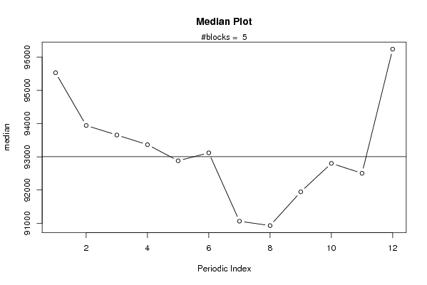
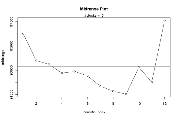
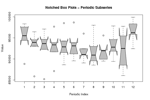
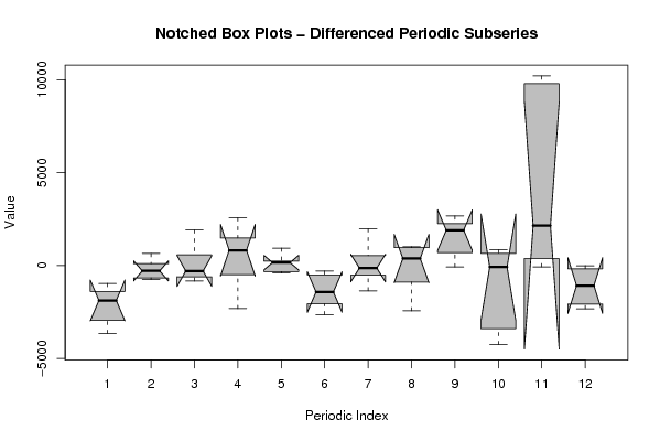
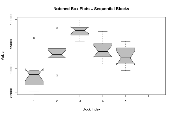
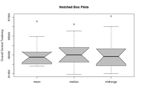
Figures (Output of Computation) | |||||||||||||||||||||
Input Parameters & R Code | |||||||||||||||||||||
| Parameters (Session): | |||||||||||||||||||||
| par1 = 12 ; | |||||||||||||||||||||
| Parameters (R input): | |||||||||||||||||||||
| par1 = 12 ; | |||||||||||||||||||||
| R code (references can be found in the software module): | |||||||||||||||||||||
par1 <- as.numeric(par1) | |||||||||||||||||||||