Repository of Reproducible Computations

Free Statistics

of Irreproducible Research!

Author's title

Author

*The author of this computation has been verified*

R Software Module

rwasp_arimaforecasting.wasp

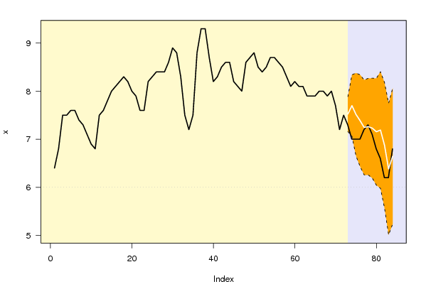
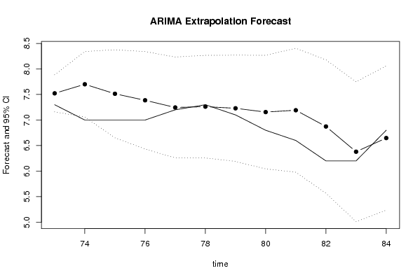
Title produced by software

ARIMA Forecasting

Date of computation

Sat, 13 Dec 2008 07:21:46 -0700

Cite this page as follows

Statistical Computations at FreeStatistics.org, Office for Research Development and Education, URL https://freestatistics.org/blog/index.php?v=date/2008/Dec/13/t1229178153jqd7hiygmmpoytd.htm/, Retrieved Sun, 19 May 2024 08:01:15 +0000

Statistical Computations at FreeStatistics.org, Office for Research Development and Education, URL https://freestatistics.org/blog/index.php?pk=33119, Retrieved Sun, 19 May 2024 08:01:15 +0000

QR Codes:

Paste this QR Code to cite your computation.

Original text written by user:

IsPrivate?

No (this computation is public)

User-defined keywords

Estimated Impact

194

Family? (F = Feedback message, R = changed R code, M = changed R Module, P = changed Parameters, D = changed Data)

-     [(Partial) Autocorrelation Function] [ACF d=0 D=0 voor Xt] [2008-12-13 09:26:24] [b1bd16d1f47bfe13feacf1c27a0abba5]
-   PD  [(Partial) Autocorrelation Function] [ACF d=0 D=1] [2008-12-13 09:29:39] [b1bd16d1f47bfe13feacf1c27a0abba5]
-   PD    [(Partial) Autocorrelation Function] [step 1 ACF d=0 D=0] [2008-12-13 13:32:41] [b1bd16d1f47bfe13feacf1c27a0abba5]
-           [(Partial) Autocorrelation Function] [step 1 ACF d=1 D=0] [2008-12-13 13:35:54] [b1bd16d1f47bfe13feacf1c27a0abba5]
-             [(Partial) Autocorrelation Function] [step 1 ACF d=1 D=1] [2008-12-13 13:38:15] [b1bd16d1f47bfe13feacf1c27a0abba5]
-               [(Partial) Autocorrelation Function] [step 1 ACF d=1 D=2] [2008-12-13 13:42:02] [b1bd16d1f47bfe13feacf1c27a0abba5]
F RM                [ARIMA Forecasting] [step 1 ARIMA fore...] [2008-12-13 14:21:46] [e7b1048c2c3a353441b9143db4404b91] [Current]

Feedback Forum

2008-12-24 10:57:26 [a2386b643d711541400692649981f2dc] [reply] 
Bij step 1 geef je een volledig antwoord waar ik niets bij kan  toevoegen. Je legt op een correcte en eenvoudig manier uit wat de parameters zijn in je tabel en je voegt er voorbeelden aan toe. 
 
Ook bij step 2, het zoeken naar een trend en seizonaliteit (grafiek 1) en de relatie tussen de voorspelling en verwachting (grafiek 2) leg je duidelijk uit! 
 
Bij step 3 vind ik dat je korter kon zijn in je antwoord. Step 3 gaan we de theoretische schatting van een gemaakte fout na. Je kon vermelden dat de p-value kleiner moet zijn dan 5% om te kunnen spreken van een significant verschil. Dit is enkel het geval in een aantal maanden. Ook kunnen we duidelijk merken dat hoe verder we zitten in de toekomst,hoe groter de fout wordt. 
 
Ik begreep niet goed wat je moest doen bij step 4 dus kan ook niet zeggen of het juist of fout is. 
 
Step 5 is ook goed beantwoord.

Post a new message

Dataseries X:

Download CSV

Histogram

Boxplots

6.4
6.8
7.5
7.5
7.6
7.6
7.4
7.3
7.1
6.9
6.8
7.5
7.6
7.8
8
8.1
8.2
8.3
8.2
8
7.9
7.6
7.6
8.2
8.3
8.4
8.4
8.4
8.6
8.9
8.8
8.3
7.5
7.2
7.5
8.8
9.3
9.3
8.7
8.2
8.3
8.5
8.6
8.6
8.2
8.1
8
8.6
8.7
8.8
8.5
8.4
8.5
8.7
8.7
8.6
8.5
8.3
8.1
8.2
8.1
8.1
7.9
7.9
7.9
8
8
7.9
8
7.7
7.2
7.5
7.3
7
7
7
7.2
7.3
7.1
6.8
6.6
6.2
6.2
6.8

Summary of computational transaction
Raw Input	view raw input (R code)
Raw Output	view raw output of R engine
Computing time	2 seconds
R Server	'George Udny Yule' @ 72.249.76.132

\begin{tabular}{lllllllll}
\hline
Summary of computational transaction \tabularnewline
Raw Input & view raw input (R code)  \tabularnewline
Raw Output & view raw output of R engine  \tabularnewline
Computing time & 2 seconds \tabularnewline
R Server & 'George Udny Yule' @ 72.249.76.132 \tabularnewline
\hline
\end{tabular}
%Source: https://freestatistics.org/blog/index.php?pk=33119&T=0

[TABLE]
[ROW][C]Summary of computational transaction[/C][/ROW]
[ROW][C]Raw Input[/C][C]view raw input (R code) [/C][/ROW]
[ROW][C]Raw Output[/C][C]view raw output of R engine [/C][/ROW]
[ROW][C]Computing time[/C][C]2 seconds[/C][/ROW]
[ROW][C]R Server[/C][C]'George Udny Yule' @ 72.249.76.132[/C][/ROW]
[/TABLE]
Source: https://freestatistics.org/blog/index.php?pk=33119&T=0

Globally Unique Identifier (entire table): ba.freestatistics.org/blog/index.php?pk=33119&T=0

As an alternative you can also use a QR Code:

The GUIDs for individual cells are displayed in the table below:

Summary of computational transaction
Raw Input	view raw input (R code)
Raw Output	view raw output of R engine
Computing time	2 seconds
R Server	'George Udny Yule' @ 72.249.76.132

Univariate ARIMA Extrapolation Forecast
time	Y[t]	F[t]	95% LB	95% UB	p-value(H0: Y[t] = F[t])	P(F[t]>Y[t-1])	P(F[t]>Y[t-s])	P(F[t]>Y[72])
60	8.2	-	-	-	-	-	-	-
61	8.1	-	-	-	-	-	-	-
62	8.1	-	-	-	-	-	-	-
63	7.9	-	-	-	-	-	-	-
64	7.9	-	-	-	-	-	-	-
65	7.9	-	-	-	-	-	-	-
66	8	-	-	-	-	-	-	-
67	8	-	-	-	-	-	-	-
68	7.9	-	-	-	-	-	-	-
69	8	-	-	-	-	-	-	-
70	7.7	-	-	-	-	-	-	-
71	7.2	-	-	-	-	-	-	-
72	7.5	-	-	-	-	-	-	-
73	7.3	7.5228	7.1598	7.8858	0.1145	0.549	9e-04	0.549
74	7	7.7003	7.0601	8.3404	0.016	0.8898	0.1105	0.7301
75	7	7.5141	6.6518	8.3764	0.1213	0.8787	0.1902	0.5128
76	7	7.3866	6.4326	8.3406	0.2135	0.7865	0.1458	0.4079
77	7.2	7.2458	6.2582	8.2334	0.4638	0.6872	0.0971	0.307
78	7.3	7.262	6.2569	8.2671	0.4705	0.5481	0.075	0.3213
79	7.1	7.23	6.1902	8.2698	0.4032	0.4475	0.0733	0.3054
80	6.8	7.156	6.0441	8.2678	0.2652	0.5393	0.0948	0.2721
81	6.6	7.1919	5.9786	8.4051	0.1695	0.7367	0.0959	0.3093
82	6.2	6.8735	5.5682	8.1788	0.1559	0.6594	0.1073	0.1734
83	6.2	6.3797	5.0104	7.749	0.3985	0.6015	0.1202	0.0544
84	6.8	6.6473	5.2351	8.0595	0.4161	0.7327	0.1183	0.1183

\begin{tabular}{lllllllll}
\hline
Univariate ARIMA Extrapolation Forecast \tabularnewline
time & Y[t] & F[t] & 95% LB & 95% UB & p-value(H0: Y[t] = F[t]) & P(F[t]>Y[t-1]) & P(F[t]>Y[t-s]) & P(F[t]>Y[72]) \tabularnewline
60 & 8.2 & - & - & - & - & - & - & - \tabularnewline
61 & 8.1 & - & - & - & - & - & - & - \tabularnewline
62 & 8.1 & - & - & - & - & - & - & - \tabularnewline
63 & 7.9 & - & - & - & - & - & - & - \tabularnewline
64 & 7.9 & - & - & - & - & - & - & - \tabularnewline
65 & 7.9 & - & - & - & - & - & - & - \tabularnewline
66 & 8 & - & - & - & - & - & - & - \tabularnewline
67 & 8 & - & - & - & - & - & - & - \tabularnewline
68 & 7.9 & - & - & - & - & - & - & - \tabularnewline
69 & 8 & - & - & - & - & - & - & - \tabularnewline
70 & 7.7 & - & - & - & - & - & - & - \tabularnewline
71 & 7.2 & - & - & - & - & - & - & - \tabularnewline
72 & 7.5 & - & - & - & - & - & - & - \tabularnewline
73 & 7.3 & 7.5228 & 7.1598 & 7.8858 & 0.1145 & 0.549 & 9e-04 & 0.549 \tabularnewline
74 & 7 & 7.7003 & 7.0601 & 8.3404 & 0.016 & 0.8898 & 0.1105 & 0.7301 \tabularnewline
75 & 7 & 7.5141 & 6.6518 & 8.3764 & 0.1213 & 0.8787 & 0.1902 & 0.5128 \tabularnewline
76 & 7 & 7.3866 & 6.4326 & 8.3406 & 0.2135 & 0.7865 & 0.1458 & 0.4079 \tabularnewline
77 & 7.2 & 7.2458 & 6.2582 & 8.2334 & 0.4638 & 0.6872 & 0.0971 & 0.307 \tabularnewline
78 & 7.3 & 7.262 & 6.2569 & 8.2671 & 0.4705 & 0.5481 & 0.075 & 0.3213 \tabularnewline
79 & 7.1 & 7.23 & 6.1902 & 8.2698 & 0.4032 & 0.4475 & 0.0733 & 0.3054 \tabularnewline
80 & 6.8 & 7.156 & 6.0441 & 8.2678 & 0.2652 & 0.5393 & 0.0948 & 0.2721 \tabularnewline
81 & 6.6 & 7.1919 & 5.9786 & 8.4051 & 0.1695 & 0.7367 & 0.0959 & 0.3093 \tabularnewline
82 & 6.2 & 6.8735 & 5.5682 & 8.1788 & 0.1559 & 0.6594 & 0.1073 & 0.1734 \tabularnewline
83 & 6.2 & 6.3797 & 5.0104 & 7.749 & 0.3985 & 0.6015 & 0.1202 & 0.0544 \tabularnewline
84 & 6.8 & 6.6473 & 5.2351 & 8.0595 & 0.4161 & 0.7327 & 0.1183 & 0.1183 \tabularnewline
\hline
\end{tabular}
%Source: https://freestatistics.org/blog/index.php?pk=33119&T=1

[TABLE]
[ROW][C]Univariate ARIMA Extrapolation Forecast[/C][/ROW]
[ROW][C]time[/C][C]Y[t][/C][C]F[t][/C][C]95% LB[/C][C]95% UB[/C][C]p-value(H0: Y[t] = F[t])[/C][C]P(F[t]>Y[t-1])[/C][C]P(F[t]>Y[t-s])[/C][C]P(F[t]>Y[72])[/C][/ROW]
[ROW][C]60[/C][C]8.2[/C][C]-[/C][C]-[/C][C]-[/C][C]-[/C][C]-[/C][C]-[/C][C]-[/C][/ROW]
[ROW][C]61[/C][C]8.1[/C][C]-[/C][C]-[/C][C]-[/C][C]-[/C][C]-[/C][C]-[/C][C]-[/C][/ROW]
[ROW][C]62[/C][C]8.1[/C][C]-[/C][C]-[/C][C]-[/C][C]-[/C][C]-[/C][C]-[/C][C]-[/C][/ROW]
[ROW][C]63[/C][C]7.9[/C][C]-[/C][C]-[/C][C]-[/C][C]-[/C][C]-[/C][C]-[/C][C]-[/C][/ROW]
[ROW][C]64[/C][C]7.9[/C][C]-[/C][C]-[/C][C]-[/C][C]-[/C][C]-[/C][C]-[/C][C]-[/C][/ROW]
[ROW][C]65[/C][C]7.9[/C][C]-[/C][C]-[/C][C]-[/C][C]-[/C][C]-[/C][C]-[/C][C]-[/C][/ROW]
[ROW][C]66[/C][C]8[/C][C]-[/C][C]-[/C][C]-[/C][C]-[/C][C]-[/C][C]-[/C][C]-[/C][/ROW]
[ROW][C]67[/C][C]8[/C][C]-[/C][C]-[/C][C]-[/C][C]-[/C][C]-[/C][C]-[/C][C]-[/C][/ROW]
[ROW][C]68[/C][C]7.9[/C][C]-[/C][C]-[/C][C]-[/C][C]-[/C][C]-[/C][C]-[/C][C]-[/C][/ROW]
[ROW][C]69[/C][C]8[/C][C]-[/C][C]-[/C][C]-[/C][C]-[/C][C]-[/C][C]-[/C][C]-[/C][/ROW]
[ROW][C]70[/C][C]7.7[/C][C]-[/C][C]-[/C][C]-[/C][C]-[/C][C]-[/C][C]-[/C][C]-[/C][/ROW]
[ROW][C]71[/C][C]7.2[/C][C]-[/C][C]-[/C][C]-[/C][C]-[/C][C]-[/C][C]-[/C][C]-[/C][/ROW]
[ROW][C]72[/C][C]7.5[/C][C]-[/C][C]-[/C][C]-[/C][C]-[/C][C]-[/C][C]-[/C][C]-[/C][/ROW]
[ROW][C]73[/C][C]7.3[/C][C]7.5228[/C][C]7.1598[/C][C]7.8858[/C][C]0.1145[/C][C]0.549[/C][C]9e-04[/C][C]0.549[/C][/ROW]
[ROW][C]74[/C][C]7[/C][C]7.7003[/C][C]7.0601[/C][C]8.3404[/C][C]0.016[/C][C]0.8898[/C][C]0.1105[/C][C]0.7301[/C][/ROW]
[ROW][C]75[/C][C]7[/C][C]7.5141[/C][C]6.6518[/C][C]8.3764[/C][C]0.1213[/C][C]0.8787[/C][C]0.1902[/C][C]0.5128[/C][/ROW]
[ROW][C]76[/C][C]7[/C][C]7.3866[/C][C]6.4326[/C][C]8.3406[/C][C]0.2135[/C][C]0.7865[/C][C]0.1458[/C][C]0.4079[/C][/ROW]
[ROW][C]77[/C][C]7.2[/C][C]7.2458[/C][C]6.2582[/C][C]8.2334[/C][C]0.4638[/C][C]0.6872[/C][C]0.0971[/C][C]0.307[/C][/ROW]
[ROW][C]78[/C][C]7.3[/C][C]7.262[/C][C]6.2569[/C][C]8.2671[/C][C]0.4705[/C][C]0.5481[/C][C]0.075[/C][C]0.3213[/C][/ROW]
[ROW][C]79[/C][C]7.1[/C][C]7.23[/C][C]6.1902[/C][C]8.2698[/C][C]0.4032[/C][C]0.4475[/C][C]0.0733[/C][C]0.3054[/C][/ROW]
[ROW][C]80[/C][C]6.8[/C][C]7.156[/C][C]6.0441[/C][C]8.2678[/C][C]0.2652[/C][C]0.5393[/C][C]0.0948[/C][C]0.2721[/C][/ROW]
[ROW][C]81[/C][C]6.6[/C][C]7.1919[/C][C]5.9786[/C][C]8.4051[/C][C]0.1695[/C][C]0.7367[/C][C]0.0959[/C][C]0.3093[/C][/ROW]
[ROW][C]82[/C][C]6.2[/C][C]6.8735[/C][C]5.5682[/C][C]8.1788[/C][C]0.1559[/C][C]0.6594[/C][C]0.1073[/C][C]0.1734[/C][/ROW]
[ROW][C]83[/C][C]6.2[/C][C]6.3797[/C][C]5.0104[/C][C]7.749[/C][C]0.3985[/C][C]0.6015[/C][C]0.1202[/C][C]0.0544[/C][/ROW]
[ROW][C]84[/C][C]6.8[/C][C]6.6473[/C][C]5.2351[/C][C]8.0595[/C][C]0.4161[/C][C]0.7327[/C][C]0.1183[/C][C]0.1183[/C][/ROW]
[/TABLE]
Source: https://freestatistics.org/blog/index.php?pk=33119&T=1

Globally Unique Identifier (entire table): ba.freestatistics.org/blog/index.php?pk=33119&T=1

As an alternative you can also use a QR Code:

The GUIDs for individual cells are displayed in the table below:

Univariate ARIMA Extrapolation Forecast
time	Y[t]	F[t]	95% LB	95% UB	p-value(H0: Y[t] = F[t])	P(F[t]>Y[t-1])	P(F[t]>Y[t-s])	P(F[t]>Y[72])
60	8.2	-	-	-	-	-	-	-
61	8.1	-	-	-	-	-	-	-
62	8.1	-	-	-	-	-	-	-
63	7.9	-	-	-	-	-	-	-
64	7.9	-	-	-	-	-	-	-
65	7.9	-	-	-	-	-	-	-
66	8	-	-	-	-	-	-	-
67	8	-	-	-	-	-	-	-
68	7.9	-	-	-	-	-	-	-
69	8	-	-	-	-	-	-	-
70	7.7	-	-	-	-	-	-	-
71	7.2	-	-	-	-	-	-	-
72	7.5	-	-	-	-	-	-	-
73	7.3	7.5228	7.1598	7.8858	0.1145	0.549	9e-04	0.549
74	7	7.7003	7.0601	8.3404	0.016	0.8898	0.1105	0.7301
75	7	7.5141	6.6518	8.3764	0.1213	0.8787	0.1902	0.5128
76	7	7.3866	6.4326	8.3406	0.2135	0.7865	0.1458	0.4079
77	7.2	7.2458	6.2582	8.2334	0.4638	0.6872	0.0971	0.307
78	7.3	7.262	6.2569	8.2671	0.4705	0.5481	0.075	0.3213
79	7.1	7.23	6.1902	8.2698	0.4032	0.4475	0.0733	0.3054
80	6.8	7.156	6.0441	8.2678	0.2652	0.5393	0.0948	0.2721
81	6.6	7.1919	5.9786	8.4051	0.1695	0.7367	0.0959	0.3093
82	6.2	6.8735	5.5682	8.1788	0.1559	0.6594	0.1073	0.1734
83	6.2	6.3797	5.0104	7.749	0.3985	0.6015	0.1202	0.0544
84	6.8	6.6473	5.2351	8.0595	0.4161	0.7327	0.1183	0.1183

Univariate ARIMA Extrapolation Forecast Performance
time	% S.E.	PE	MAPE	Sq.E	MSE	RMSE
73	0.0246	-0.0296	0.0025	0.0496	0.0041	0.0643
74	0.0424	-0.0909	0.0076	0.4904	0.0409	0.2021
75	0.0586	-0.0684	0.0057	0.2643	0.022	0.1484
76	0.0659	-0.0523	0.0044	0.1495	0.0125	0.1116
77	0.0695	-0.0063	5e-04	0.0021	2e-04	0.0132
78	0.0706	0.0052	4e-04	0.0014	1e-04	0.011
79	0.0734	-0.018	0.0015	0.0169	0.0014	0.0375
80	0.0793	-0.0497	0.0041	0.1267	0.0106	0.1028
81	0.0861	-0.0823	0.0069	0.3503	0.0292	0.1709
82	0.0969	-0.098	0.0082	0.4537	0.0378	0.1944
83	0.1095	-0.0282	0.0023	0.0323	0.0027	0.0519
84	0.1084	0.023	0.0019	0.0233	0.0019	0.0441

\begin{tabular}{lllllllll}
\hline
Univariate ARIMA Extrapolation Forecast Performance \tabularnewline
time & % S.E. & PE & MAPE & Sq.E & MSE & RMSE \tabularnewline
73 & 0.0246 & -0.0296 & 0.0025 & 0.0496 & 0.0041 & 0.0643 \tabularnewline
74 & 0.0424 & -0.0909 & 0.0076 & 0.4904 & 0.0409 & 0.2021 \tabularnewline
75 & 0.0586 & -0.0684 & 0.0057 & 0.2643 & 0.022 & 0.1484 \tabularnewline
76 & 0.0659 & -0.0523 & 0.0044 & 0.1495 & 0.0125 & 0.1116 \tabularnewline
77 & 0.0695 & -0.0063 & 5e-04 & 0.0021 & 2e-04 & 0.0132 \tabularnewline
78 & 0.0706 & 0.0052 & 4e-04 & 0.0014 & 1e-04 & 0.011 \tabularnewline
79 & 0.0734 & -0.018 & 0.0015 & 0.0169 & 0.0014 & 0.0375 \tabularnewline
80 & 0.0793 & -0.0497 & 0.0041 & 0.1267 & 0.0106 & 0.1028 \tabularnewline
81 & 0.0861 & -0.0823 & 0.0069 & 0.3503 & 0.0292 & 0.1709 \tabularnewline
82 & 0.0969 & -0.098 & 0.0082 & 0.4537 & 0.0378 & 0.1944 \tabularnewline
83 & 0.1095 & -0.0282 & 0.0023 & 0.0323 & 0.0027 & 0.0519 \tabularnewline
84 & 0.1084 & 0.023 & 0.0019 & 0.0233 & 0.0019 & 0.0441 \tabularnewline
\hline
\end{tabular}
%Source: https://freestatistics.org/blog/index.php?pk=33119&T=2

[TABLE]
[ROW][C]Univariate ARIMA Extrapolation Forecast Performance[/C][/ROW]
[ROW][C]time[/C][C]% S.E.[/C][C]PE[/C][C]MAPE[/C][C]Sq.E[/C][C]MSE[/C][C]RMSE[/C][/ROW]
[ROW][C]73[/C][C]0.0246[/C][C]-0.0296[/C][C]0.0025[/C][C]0.0496[/C][C]0.0041[/C][C]0.0643[/C][/ROW]
[ROW][C]74[/C][C]0.0424[/C][C]-0.0909[/C][C]0.0076[/C][C]0.4904[/C][C]0.0409[/C][C]0.2021[/C][/ROW]
[ROW][C]75[/C][C]0.0586[/C][C]-0.0684[/C][C]0.0057[/C][C]0.2643[/C][C]0.022[/C][C]0.1484[/C][/ROW]
[ROW][C]76[/C][C]0.0659[/C][C]-0.0523[/C][C]0.0044[/C][C]0.1495[/C][C]0.0125[/C][C]0.1116[/C][/ROW]
[ROW][C]77[/C][C]0.0695[/C][C]-0.0063[/C][C]5e-04[/C][C]0.0021[/C][C]2e-04[/C][C]0.0132[/C][/ROW]
[ROW][C]78[/C][C]0.0706[/C][C]0.0052[/C][C]4e-04[/C][C]0.0014[/C][C]1e-04[/C][C]0.011[/C][/ROW]
[ROW][C]79[/C][C]0.0734[/C][C]-0.018[/C][C]0.0015[/C][C]0.0169[/C][C]0.0014[/C][C]0.0375[/C][/ROW]
[ROW][C]80[/C][C]0.0793[/C][C]-0.0497[/C][C]0.0041[/C][C]0.1267[/C][C]0.0106[/C][C]0.1028[/C][/ROW]
[ROW][C]81[/C][C]0.0861[/C][C]-0.0823[/C][C]0.0069[/C][C]0.3503[/C][C]0.0292[/C][C]0.1709[/C][/ROW]
[ROW][C]82[/C][C]0.0969[/C][C]-0.098[/C][C]0.0082[/C][C]0.4537[/C][C]0.0378[/C][C]0.1944[/C][/ROW]
[ROW][C]83[/C][C]0.1095[/C][C]-0.0282[/C][C]0.0023[/C][C]0.0323[/C][C]0.0027[/C][C]0.0519[/C][/ROW]
[ROW][C]84[/C][C]0.1084[/C][C]0.023[/C][C]0.0019[/C][C]0.0233[/C][C]0.0019[/C][C]0.0441[/C][/ROW]
[/TABLE]
Source: https://freestatistics.org/blog/index.php?pk=33119&T=2

Globally Unique Identifier (entire table): ba.freestatistics.org/blog/index.php?pk=33119&T=2

As an alternative you can also use a QR Code:

The GUIDs for individual cells are displayed in the table below:

Univariate ARIMA Extrapolation Forecast Performance
time	% S.E.	PE	MAPE	Sq.E	MSE	RMSE
73	0.0246	-0.0296	0.0025	0.0496	0.0041	0.0643
74	0.0424	-0.0909	0.0076	0.4904	0.0409	0.2021
75	0.0586	-0.0684	0.0057	0.2643	0.022	0.1484
76	0.0659	-0.0523	0.0044	0.1495	0.0125	0.1116
77	0.0695	-0.0063	5e-04	0.0021	2e-04	0.0132
78	0.0706	0.0052	4e-04	0.0014	1e-04	0.011
79	0.0734	-0.018	0.0015	0.0169	0.0014	0.0375
80	0.0793	-0.0497	0.0041	0.1267	0.0106	0.1028
81	0.0861	-0.0823	0.0069	0.3503	0.0292	0.1709
82	0.0969	-0.098	0.0082	0.4537	0.0378	0.1944
83	0.1095	-0.0282	0.0023	0.0323	0.0027	0.0519
84	0.1084	0.023	0.0019	0.0233	0.0019	0.0441

Figure 1

PNG link

Postscript link

PDF link

Figure 2

PNG link

Postscript link

PDF link

Parameters (Session):

par1 = 1 ; par2 = 0 ; par3 = 2 ; par4 = 12 ;

Parameters (R input):

par1 = 12 ; par2 = 1 ; par3 = 2 ; par4 = 1 ; par5 = 12 ; par6 = 3 ; par7 = 1 ; par8 = 1 ; par9 = 1 ; par10 = FALSE ;

R code (references can be found in the software module):

par1 <- as.numeric(par1) #cut off periods
par2 <- as.numeric(par2) #lambda
par3 <- as.numeric(par3) #degree of non-seasonal differencing
par4 <- as.numeric(par4) #degree of seasonal differencing
par5 <- as.numeric(par5) #seasonal period
par6 <- as.numeric(par6) #p
par7 <- as.numeric(par7) #q
par8 <- as.numeric(par8) #P
par9 <- as.numeric(par9) #Q
if (par10 == 'TRUE') par10 <- TRUE
if (par10 == 'FALSE') par10 <- FALSE
if (par2 == 0) x <- log(x)
if (par2 != 0) x <- x^par2
lx <- length(x)
first <- lx - 2*par1
nx <- lx - par1
nx1 <- nx + 1
fx <- lx - nx
if (fx < 1) {
fx <- par5
nx1 <- lx + fx - 1
first <- lx - 2*fx
}
first <- 1
if (fx < 3) fx <- round(lx/10,0)
(arima.out <- arima(x[1:nx], order=c(par6,par3,par7), seasonal=list(order=c(par8,par4,par9), period=par5), include.mean=par10, method='ML'))
(forecast <- predict(arima.out,fx))
(lb <- forecast$pred - 1.96 * forecast$se)
(ub <- forecast$pred + 1.96 * forecast$se)
if (par2 == 0) {
x <- exp(x)
forecast$pred <- exp(forecast$pred)
lb <- exp(lb)
ub <- exp(ub)
}
if (par2 != 0) {
x <- x^(1/par2)
forecast$pred <- forecast$pred^(1/par2)
lb <- lb^(1/par2)
ub <- ub^(1/par2)
}
if (par2 < 0) {
olb <- lb
lb <- ub
ub <- olb
}
(actandfor <- c(x[1:nx], forecast$pred))
(perc.se <- (ub-forecast$pred)/1.96/forecast$pred)
bitmap(file='test1.png')
opar <- par(mar=c(4,4,2,2),las=1)
ylim <- c( min(x[first:nx],lb), max(x[first:nx],ub))
plot(x,ylim=ylim,type='n',xlim=c(first,lx))
usr <- par('usr')
rect(usr[1],usr[3],nx+1,usr[4],border=NA,col='lemonchiffon')
rect(nx1,usr[3],usr[2],usr[4],border=NA,col='lavender')
abline(h= (-3:3)*2 , col ='gray', lty =3)
polygon( c(nx1:lx,lx:nx1), c(lb,rev(ub)), col = 'orange', lty=2,border=NA)
lines(nx1:lx, lb , lty=2)
lines(nx1:lx, ub , lty=2)
lines(x, lwd=2)
lines(nx1:lx, forecast$pred , lwd=2 , col ='white')
box()
par(opar)
dev.off()
prob.dec <- array(NA, dim=fx)
prob.sdec <- array(NA, dim=fx)
prob.ldec <- array(NA, dim=fx)
prob.pval <- array(NA, dim=fx)
perf.pe <- array(0, dim=fx)
perf.mape <- array(0, dim=fx)
perf.se <- array(0, dim=fx)
perf.mse <- array(0, dim=fx)
perf.rmse <- array(0, dim=fx)
for (i in 1:fx) {
locSD <- (ub[i] - forecast$pred[i]) / 1.96
perf.pe[i] = (x[nx+i] - forecast$pred[i]) / forecast$pred[i]
perf.mape[i] = perf.mape[i] + abs(perf.pe[i])
perf.se[i] = (x[nx+i] - forecast$pred[i])^2
perf.mse[i] = perf.mse[i] + perf.se[i]
prob.dec[i] = pnorm((x[nx+i-1] - forecast$pred[i]) / locSD)
prob.sdec[i] = pnorm((x[nx+i-par5] - forecast$pred[i]) / locSD)
prob.ldec[i] = pnorm((x[nx] - forecast$pred[i]) / locSD)
prob.pval[i] = pnorm(abs(x[nx+i] - forecast$pred[i]) / locSD)
}
perf.mape = perf.mape / fx
perf.mse = perf.mse / fx
perf.rmse = sqrt(perf.mse)
bitmap(file='test2.png')
plot(forecast$pred, pch=19, type='b',main='ARIMA Extrapolation Forecast', ylab='Forecast and 95% CI', xlab='time',ylim=c(min(lb),max(ub)))
dum <- forecast$pred
dum[1:12] <- x[(nx+1):lx]
lines(dum, lty=1)
lines(ub,lty=3)
lines(lb,lty=3)
dev.off()
load(file='createtable')
a<-table.start()
a<-table.row.start(a)
a<-table.element(a,'Univariate ARIMA Extrapolation Forecast',9,TRUE)
a<-table.row.end(a)
a<-table.row.start(a)
a<-table.element(a,'time',1,header=TRUE)
a<-table.element(a,'Y[t]',1,header=TRUE)
a<-table.element(a,'F[t]',1,header=TRUE)
a<-table.element(a,'95% LB',1,header=TRUE)
a<-table.element(a,'95% UB',1,header=TRUE)
a<-table.element(a,'p-value
(H0: Y[t] = F[t])',1,header=TRUE)
a<-table.element(a,'P(F[t]>Y[t-1])',1,header=TRUE)
a<-table.element(a,'P(F[t]>Y[t-s])',1,header=TRUE)
mylab <- paste('P(F[t]>Y[',nx,sep='')
mylab <- paste(mylab,'])',sep='')
a<-table.element(a,mylab,1,header=TRUE)
a<-table.row.end(a)
for (i in (nx-par5):nx) {
a<-table.row.start(a)
a<-table.element(a,i,header=TRUE)
a<-table.element(a,x[i])
a<-table.element(a,'-')
a<-table.element(a,'-')
a<-table.element(a,'-')
a<-table.element(a,'-')
a<-table.element(a,'-')
a<-table.element(a,'-')
a<-table.element(a,'-')
a<-table.row.end(a)
}
for (i in 1:fx) {
a<-table.row.start(a)
a<-table.element(a,nx+i,header=TRUE)
a<-table.element(a,round(x[nx+i],4))
a<-table.element(a,round(forecast$pred[i],4))
a<-table.element(a,round(lb[i],4))
a<-table.element(a,round(ub[i],4))
a<-table.element(a,round((1-prob.pval[i]),4))
a<-table.element(a,round((1-prob.dec[i]),4))
a<-table.element(a,round((1-prob.sdec[i]),4))
a<-table.element(a,round((1-prob.ldec[i]),4))
a<-table.row.end(a)
}
a<-table.end(a)
table.save(a,file='mytable.tab')
a<-table.start()
a<-table.row.start(a)
a<-table.element(a,'Univariate ARIMA Extrapolation Forecast Performance',7,TRUE)
a<-table.row.end(a)
a<-table.row.start(a)
a<-table.element(a,'time',1,header=TRUE)
a<-table.element(a,'% S.E.',1,header=TRUE)
a<-table.element(a,'PE',1,header=TRUE)
a<-table.element(a,'MAPE',1,header=TRUE)
a<-table.element(a,'Sq.E',1,header=TRUE)
a<-table.element(a,'MSE',1,header=TRUE)
a<-table.element(a,'RMSE',1,header=TRUE)
a<-table.row.end(a)
for (i in 1:fx) {
a<-table.row.start(a)
a<-table.element(a,nx+i,header=TRUE)
a<-table.element(a,round(perc.se[i],4))
a<-table.element(a,round(perf.pe[i],4))
a<-table.element(a,round(perf.mape[i],4))
a<-table.element(a,round(perf.se[i],4))
a<-table.element(a,round(perf.mse[i],4))
a<-table.element(a,round(perf.rmse[i],4))
a<-table.row.end(a)
}
a<-table.end(a)
table.save(a,file='mytable1.tab')

Free Statistics

Description of Statistical Computation

Tree of Dependent Computations

Dataset

Tables (Output of Computation)

Figures (Output of Computation)

Input Parameters & R Code