Repository of Reproducible Computations

Free Statistics

of Irreproducible Research!

Author's title

Author

*The author of this computation has been verified*

R Software Module

rwasp_autocorrelation.wasp

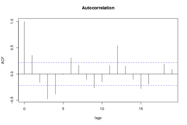
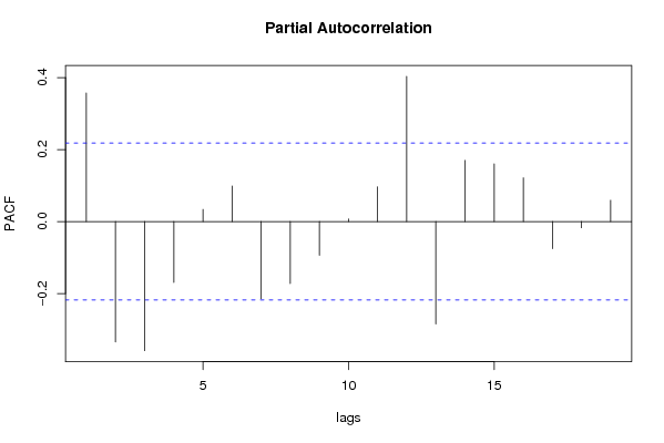
Title produced by software

(Partial) Autocorrelation Function

Date of computation

Sat, 13 Dec 2008 05:15:31 -0700

Cite this page as follows

Statistical Computations at FreeStatistics.org, Office for Research Development and Education, URL https://freestatistics.org/blog/index.php?v=date/2008/Dec/13/t1229170571s068bv0w0pcu8jq.htm/, Retrieved Mon, 27 May 2024 12:12:32 +0000

Statistical Computations at FreeStatistics.org, Office for Research Development and Education, URL https://freestatistics.org/blog/index.php?pk=33000, Retrieved Mon, 27 May 2024 12:12:32 +0000

QR Codes:

Paste this QR Code to cite your computation.

Original text written by user:

IsPrivate?

No (this computation is public)

User-defined keywords

jenske_cole@hotmail.com

Estimated Impact

171

Family? (F = Feedback message, R = changed R code, M = changed R Module, P = changed Parameters, D = changed Data)

F     [Bivariate Kernel Density Estimation] [Various EDA Topic...] [2008-11-12 13:37:39] [8094ad203a218aaca2d1cea2c78c2d6e]
F    D  [Bivariate Kernel Density Estimation] [opdracht3 blok8 q...] [2008-11-12 17:51:49] [975daa21de49eaf4d491226310243f5a]
- RMPD      [(Partial) Autocorrelation Function] [paper autocorrela...] [2008-12-13 12:15:31] [120dfa2440e51a0cfc0f5296bc5d7460] [Current]
-             [(Partial) Autocorrelation Function] [paper autocorrela...] [2008-12-13 13:03:08] [975daa21de49eaf4d491226310243f5a] 
-             [(Partial) Autocorrelation Function] [paper autocorrela...] [2008-12-13 13:04:42] [975daa21de49eaf4d491226310243f5a] 
-             [(Partial) Autocorrelation Function] [paper autocorrela...] [2008-12-13 13:06:03] [975daa21de49eaf4d491226310243f5a] 

Feedback Forum

Post a new message

Dataseries X:

Download CSV

Histogram

Boxplots

7.6
7.4
7.3
7.1
6.9
6.8
7.5
7.6
7.8
8
8.1
8.2
8.3
8.2
8
7.9
7.6
7.6
8.2
8.3
8.4
8.4
8.4
8.6
8.9
8.8
8.3
7.5
7.2
7.5
8.8
9.3
9.3
8.7
8.2
8.3
8.5
8.6
8.6
8.2
8.1
8
8.6
8.7
8.8
8.5
8.4
8.5
8.7
8.7
8.6
8.5
8.3
8.1
8.2
8.1
8.1
7.9
7.9
7.9
8
8
7.9
8
7.7
7.2
7.5
7.3
7
7
7
7.2
7.3
7.1
6.8
6.6
6.2
6.2
6.8
6.9
6.8
6.7

Summary of computational transaction
Raw Input	view raw input (R code)
Raw Output	view raw output of R engine
Computing time	2 seconds
R Server	'Sir Ronald Aylmer Fisher' @ 193.190.124.24

\begin{tabular}{lllllllll}
\hline
Summary of computational transaction \tabularnewline
Raw Input & view raw input (R code)  \tabularnewline
Raw Output & view raw output of R engine  \tabularnewline
Computing time & 2 seconds \tabularnewline
R Server & 'Sir Ronald Aylmer Fisher' @ 193.190.124.24 \tabularnewline
\hline
\end{tabular}
%Source: https://freestatistics.org/blog/index.php?pk=33000&T=0

[TABLE]
[ROW][C]Summary of computational transaction[/C][/ROW]
[ROW][C]Raw Input[/C][C]view raw input (R code) [/C][/ROW]
[ROW][C]Raw Output[/C][C]view raw output of R engine [/C][/ROW]
[ROW][C]Computing time[/C][C]2 seconds[/C][/ROW]
[ROW][C]R Server[/C][C]'Sir Ronald Aylmer Fisher' @ 193.190.124.24[/C][/ROW]
[/TABLE]
Source: https://freestatistics.org/blog/index.php?pk=33000&T=0

Globally Unique Identifier (entire table): ba.freestatistics.org/blog/index.php?pk=33000&T=0

As an alternative you can also use a QR Code:

The GUIDs for individual cells are displayed in the table below:

Summary of computational transaction
Raw Input	view raw input (R code)
Raw Output	view raw output of R engine
Computing time	2 seconds
R Server	'Sir Ronald Aylmer Fisher' @ 193.190.124.24

Autocorrelation Function
Time lag k	ACF(k)	T-STAT	P-value
1	0.356996	3.213	0.000943
2	-0.164575	-1.4812	0.071219
3	-0.475916	-4.2832	2.5e-05
4	-0.38501	-3.4651	0.000425
5	-0.011924	-0.1073	0.457402
6	0.311374	2.8024	0.003172
7	0.168067	1.5126	0.067137
8	-0.105023	-0.9452	0.173683
9	-0.267608	-2.4085	0.009145
10	-0.149076	-1.3417	0.091724
11	0.161927	1.4573	0.074443
12	0.54154	4.8739	3e-06
13	0.155063	1.3956	0.083329
14	-0.10649	-0.9584	0.170354
15	-0.278183	-2.5036	0.007151
16	-0.194866	-1.7538	0.041624
17	0.002597	0.0234	0.490704
18	0.187917	1.6913	0.047316
19	0.090602	0.8154	0.208611

\begin{tabular}{lllllllll}
\hline
Autocorrelation Function \tabularnewline
Time lag k & ACF(k) & T-STAT & P-value \tabularnewline
1 & 0.356996 & 3.213 & 0.000943 \tabularnewline
2 & -0.164575 & -1.4812 & 0.071219 \tabularnewline
3 & -0.475916 & -4.2832 & 2.5e-05 \tabularnewline
4 & -0.38501 & -3.4651 & 0.000425 \tabularnewline
5 & -0.011924 & -0.1073 & 0.457402 \tabularnewline
6 & 0.311374 & 2.8024 & 0.003172 \tabularnewline
7 & 0.168067 & 1.5126 & 0.067137 \tabularnewline
8 & -0.105023 & -0.9452 & 0.173683 \tabularnewline
9 & -0.267608 & -2.4085 & 0.009145 \tabularnewline
10 & -0.149076 & -1.3417 & 0.091724 \tabularnewline
11 & 0.161927 & 1.4573 & 0.074443 \tabularnewline
12 & 0.54154 & 4.8739 & 3e-06 \tabularnewline
13 & 0.155063 & 1.3956 & 0.083329 \tabularnewline
14 & -0.10649 & -0.9584 & 0.170354 \tabularnewline
15 & -0.278183 & -2.5036 & 0.007151 \tabularnewline
16 & -0.194866 & -1.7538 & 0.041624 \tabularnewline
17 & 0.002597 & 0.0234 & 0.490704 \tabularnewline
18 & 0.187917 & 1.6913 & 0.047316 \tabularnewline
19 & 0.090602 & 0.8154 & 0.208611 \tabularnewline
\hline
\end{tabular}
%Source: https://freestatistics.org/blog/index.php?pk=33000&T=1

[TABLE]
[ROW][C]Autocorrelation Function[/C][/ROW]
[ROW][C]Time lag k[/C][C]ACF(k)[/C][C]T-STAT[/C][C]P-value[/C][/ROW]
[ROW][C]1[/C][C]0.356996[/C][C]3.213[/C][C]0.000943[/C][/ROW]
[ROW][C]2[/C][C]-0.164575[/C][C]-1.4812[/C][C]0.071219[/C][/ROW]
[ROW][C]3[/C][C]-0.475916[/C][C]-4.2832[/C][C]2.5e-05[/C][/ROW]
[ROW][C]4[/C][C]-0.38501[/C][C]-3.4651[/C][C]0.000425[/C][/ROW]
[ROW][C]5[/C][C]-0.011924[/C][C]-0.1073[/C][C]0.457402[/C][/ROW]
[ROW][C]6[/C][C]0.311374[/C][C]2.8024[/C][C]0.003172[/C][/ROW]
[ROW][C]7[/C][C]0.168067[/C][C]1.5126[/C][C]0.067137[/C][/ROW]
[ROW][C]8[/C][C]-0.105023[/C][C]-0.9452[/C][C]0.173683[/C][/ROW]
[ROW][C]9[/C][C]-0.267608[/C][C]-2.4085[/C][C]0.009145[/C][/ROW]
[ROW][C]10[/C][C]-0.149076[/C][C]-1.3417[/C][C]0.091724[/C][/ROW]
[ROW][C]11[/C][C]0.161927[/C][C]1.4573[/C][C]0.074443[/C][/ROW]
[ROW][C]12[/C][C]0.54154[/C][C]4.8739[/C][C]3e-06[/C][/ROW]
[ROW][C]13[/C][C]0.155063[/C][C]1.3956[/C][C]0.083329[/C][/ROW]
[ROW][C]14[/C][C]-0.10649[/C][C]-0.9584[/C][C]0.170354[/C][/ROW]
[ROW][C]15[/C][C]-0.278183[/C][C]-2.5036[/C][C]0.007151[/C][/ROW]
[ROW][C]16[/C][C]-0.194866[/C][C]-1.7538[/C][C]0.041624[/C][/ROW]
[ROW][C]17[/C][C]0.002597[/C][C]0.0234[/C][C]0.490704[/C][/ROW]
[ROW][C]18[/C][C]0.187917[/C][C]1.6913[/C][C]0.047316[/C][/ROW]
[ROW][C]19[/C][C]0.090602[/C][C]0.8154[/C][C]0.208611[/C][/ROW]
[/TABLE]
Source: https://freestatistics.org/blog/index.php?pk=33000&T=1

Globally Unique Identifier (entire table): ba.freestatistics.org/blog/index.php?pk=33000&T=1

As an alternative you can also use a QR Code:

The GUIDs for individual cells are displayed in the table below:

Autocorrelation Function
Time lag k	ACF(k)	T-STAT	P-value
1	0.356996	3.213	0.000943
2	-0.164575	-1.4812	0.071219
3	-0.475916	-4.2832	2.5e-05
4	-0.38501	-3.4651	0.000425
5	-0.011924	-0.1073	0.457402
6	0.311374	2.8024	0.003172
7	0.168067	1.5126	0.067137
8	-0.105023	-0.9452	0.173683
9	-0.267608	-2.4085	0.009145
10	-0.149076	-1.3417	0.091724
11	0.161927	1.4573	0.074443
12	0.54154	4.8739	3e-06
13	0.155063	1.3956	0.083329
14	-0.10649	-0.9584	0.170354
15	-0.278183	-2.5036	0.007151
16	-0.194866	-1.7538	0.041624
17	0.002597	0.0234	0.490704
18	0.187917	1.6913	0.047316
19	0.090602	0.8154	0.208611

Partial Autocorrelation Function
Time lag k	PACF(k)	T-STAT	P-value
1	0.356996	3.213	0.000943
2	-0.334674	-3.0121	0.00173
3	-0.358821	-3.2294	0.000896
4	-0.169236	-1.5231	0.065811
5	0.033706	0.3034	0.381199
6	0.09867	0.888	0.188577
7	-0.214886	-1.934	0.028304
8	-0.172587	-1.5533	0.062127
9	-0.093911	-0.8452	0.200244
10	0.007036	0.0633	0.474831
11	0.096132	0.8652	0.194746
12	0.403256	3.6293	0.000248
13	-0.284446	-2.56	0.006163
14	0.169688	1.5272	0.065305
15	0.160302	1.4427	0.076478
16	0.121361	1.0923	0.13898
17	-0.075167	-0.6765	0.250325
18	-0.017289	-0.1556	0.438367
19	0.058959	0.5306	0.298564

\begin{tabular}{lllllllll}
\hline
Partial Autocorrelation Function \tabularnewline
Time lag k & PACF(k) & T-STAT & P-value \tabularnewline
1 & 0.356996 & 3.213 & 0.000943 \tabularnewline
2 & -0.334674 & -3.0121 & 0.00173 \tabularnewline
3 & -0.358821 & -3.2294 & 0.000896 \tabularnewline
4 & -0.169236 & -1.5231 & 0.065811 \tabularnewline
5 & 0.033706 & 0.3034 & 0.381199 \tabularnewline
6 & 0.09867 & 0.888 & 0.188577 \tabularnewline
7 & -0.214886 & -1.934 & 0.028304 \tabularnewline
8 & -0.172587 & -1.5533 & 0.062127 \tabularnewline
9 & -0.093911 & -0.8452 & 0.200244 \tabularnewline
10 & 0.007036 & 0.0633 & 0.474831 \tabularnewline
11 & 0.096132 & 0.8652 & 0.194746 \tabularnewline
12 & 0.403256 & 3.6293 & 0.000248 \tabularnewline
13 & -0.284446 & -2.56 & 0.006163 \tabularnewline
14 & 0.169688 & 1.5272 & 0.065305 \tabularnewline
15 & 0.160302 & 1.4427 & 0.076478 \tabularnewline
16 & 0.121361 & 1.0923 & 0.13898 \tabularnewline
17 & -0.075167 & -0.6765 & 0.250325 \tabularnewline
18 & -0.017289 & -0.1556 & 0.438367 \tabularnewline
19 & 0.058959 & 0.5306 & 0.298564 \tabularnewline
\hline
\end{tabular}
%Source: https://freestatistics.org/blog/index.php?pk=33000&T=2

[TABLE]
[ROW][C]Partial Autocorrelation Function[/C][/ROW]
[ROW][C]Time lag k[/C][C]PACF(k)[/C][C]T-STAT[/C][C]P-value[/C][/ROW]
[ROW][C]1[/C][C]0.356996[/C][C]3.213[/C][C]0.000943[/C][/ROW]
[ROW][C]2[/C][C]-0.334674[/C][C]-3.0121[/C][C]0.00173[/C][/ROW]
[ROW][C]3[/C][C]-0.358821[/C][C]-3.2294[/C][C]0.000896[/C][/ROW]
[ROW][C]4[/C][C]-0.169236[/C][C]-1.5231[/C][C]0.065811[/C][/ROW]
[ROW][C]5[/C][C]0.033706[/C][C]0.3034[/C][C]0.381199[/C][/ROW]
[ROW][C]6[/C][C]0.09867[/C][C]0.888[/C][C]0.188577[/C][/ROW]
[ROW][C]7[/C][C]-0.214886[/C][C]-1.934[/C][C]0.028304[/C][/ROW]
[ROW][C]8[/C][C]-0.172587[/C][C]-1.5533[/C][C]0.062127[/C][/ROW]
[ROW][C]9[/C][C]-0.093911[/C][C]-0.8452[/C][C]0.200244[/C][/ROW]
[ROW][C]10[/C][C]0.007036[/C][C]0.0633[/C][C]0.474831[/C][/ROW]
[ROW][C]11[/C][C]0.096132[/C][C]0.8652[/C][C]0.194746[/C][/ROW]
[ROW][C]12[/C][C]0.403256[/C][C]3.6293[/C][C]0.000248[/C][/ROW]
[ROW][C]13[/C][C]-0.284446[/C][C]-2.56[/C][C]0.006163[/C][/ROW]
[ROW][C]14[/C][C]0.169688[/C][C]1.5272[/C][C]0.065305[/C][/ROW]
[ROW][C]15[/C][C]0.160302[/C][C]1.4427[/C][C]0.076478[/C][/ROW]
[ROW][C]16[/C][C]0.121361[/C][C]1.0923[/C][C]0.13898[/C][/ROW]
[ROW][C]17[/C][C]-0.075167[/C][C]-0.6765[/C][C]0.250325[/C][/ROW]
[ROW][C]18[/C][C]-0.017289[/C][C]-0.1556[/C][C]0.438367[/C][/ROW]
[ROW][C]19[/C][C]0.058959[/C][C]0.5306[/C][C]0.298564[/C][/ROW]
[/TABLE]
Source: https://freestatistics.org/blog/index.php?pk=33000&T=2

Globally Unique Identifier (entire table): ba.freestatistics.org/blog/index.php?pk=33000&T=2

As an alternative you can also use a QR Code:

The GUIDs for individual cells are displayed in the table below:

Partial Autocorrelation Function
Time lag k	PACF(k)	T-STAT	P-value
1	0.356996	3.213	0.000943
2	-0.334674	-3.0121	0.00173
3	-0.358821	-3.2294	0.000896
4	-0.169236	-1.5231	0.065811
5	0.033706	0.3034	0.381199
6	0.09867	0.888	0.188577
7	-0.214886	-1.934	0.028304
8	-0.172587	-1.5533	0.062127
9	-0.093911	-0.8452	0.200244
10	0.007036	0.0633	0.474831
11	0.096132	0.8652	0.194746
12	0.403256	3.6293	0.000248
13	-0.284446	-2.56	0.006163
14	0.169688	1.5272	0.065305
15	0.160302	1.4427	0.076478
16	0.121361	1.0923	0.13898
17	-0.075167	-0.6765	0.250325
18	-0.017289	-0.1556	0.438367
19	0.058959	0.5306	0.298564

Figure 1

PNG link

Postscript link

PDF link

Figure 2

PNG link

Postscript link

PDF link

Parameters (Session):

par1 = 4 ;

Parameters (R input):

par1 = Default ; par2 = 1 ; par3 = 1 ; par4 = 0 ; par5 = 12 ;

R code (references can be found in the software module):

if (par1 == 'Default') {
par1 = 10*log10(length(x))
} else {
par1 <- as.numeric(par1)
}
par2 <- as.numeric(par2)
par3 <- as.numeric(par3)
par4 <- as.numeric(par4)
par5 <- as.numeric(par5)
if (par2 == 0) {
x <- log(x)
} else {
x <- (x ^ par2 - 1) / par2
}
if (par3 > 0) x <- diff(x,lag=1,difference=par3)
if (par4 > 0) x <- diff(x,lag=par5,difference=par4)
bitmap(file='pic1.png')
racf <- acf(x,par1,main='Autocorrelation',xlab='lags',ylab='ACF')
dev.off()
bitmap(file='pic2.png')
rpacf <- pacf(x,par1,main='Partial Autocorrelation',xlab='lags',ylab='PACF')
dev.off()
(myacf <- c(racf$acf))
(mypacf <- c(rpacf$acf))
lengthx <- length(x)
sqrtn <- sqrt(lengthx)
load(file='createtable')
a<-table.start()
a<-table.row.start(a)
a<-table.element(a,'Autocorrelation Function',4,TRUE)
a<-table.row.end(a)
a<-table.row.start(a)
a<-table.element(a,'Time lag k',header=TRUE)
a<-table.element(a,hyperlink('basics.htm','ACF(k)','click here for more information about the Autocorrelation Function'),header=TRUE)
a<-table.element(a,'T-STAT',header=TRUE)
a<-table.element(a,'P-value',header=TRUE)
a<-table.row.end(a)
for (i in 2:(par1+1)) {
a<-table.row.start(a)
a<-table.element(a,i-1,header=TRUE)
a<-table.element(a,round(myacf[i],6))
mytstat <- myacf[i]*sqrtn
a<-table.element(a,round(mytstat,4))
a<-table.element(a,round(1-pt(abs(mytstat),lengthx),6))
a<-table.row.end(a)
}
a<-table.end(a)
table.save(a,file='mytable.tab')
a<-table.start()
a<-table.row.start(a)
a<-table.element(a,'Partial Autocorrelation Function',4,TRUE)
a<-table.row.end(a)
a<-table.row.start(a)
a<-table.element(a,'Time lag k',header=TRUE)
a<-table.element(a,hyperlink('basics.htm','PACF(k)','click here for more information about the Partial Autocorrelation Function'),header=TRUE)
a<-table.element(a,'T-STAT',header=TRUE)
a<-table.element(a,'P-value',header=TRUE)
a<-table.row.end(a)
for (i in 1:par1) {
a<-table.row.start(a)
a<-table.element(a,i,header=TRUE)
a<-table.element(a,round(mypacf[i],6))
mytstat <- mypacf[i]*sqrtn
a<-table.element(a,round(mytstat,4))
a<-table.element(a,round(1-pt(abs(mytstat),lengthx),6))
a<-table.row.end(a)
}
a<-table.end(a)
table.save(a,file='mytable1.tab')

Free Statistics

Description of Statistical Computation

Tree of Dependent Computations

Dataset

Tables (Output of Computation)

Figures (Output of Computation)

Input Parameters & R Code