Repository of Reproducible Computations

Free Statistics

of Irreproducible Research!

Author's title

Author

*The author of this computation has been verified*

R Software Module

rwasp_autocorrelation.wasp

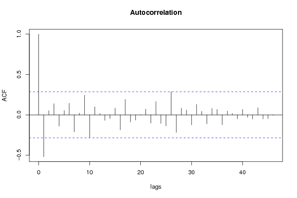
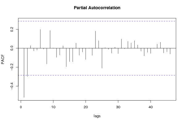
Title produced by software

(Partial) Autocorrelation Function

Date of computation

Fri, 12 Dec 2008 08:21:21 -0700

Cite this page as follows

Statistical Computations at FreeStatistics.org, Office for Research Development and Education, URL https://freestatistics.org/blog/index.php?v=date/2008/Dec/12/t1229095379tdgvi90kubosjvq.htm/, Retrieved Sun, 19 May 2024 06:05:22 +0000

Statistical Computations at FreeStatistics.org, Office for Research Development and Education, URL https://freestatistics.org/blog/index.php?pk=32844, Retrieved Sun, 19 May 2024 06:05:22 +0000

QR Codes:

Paste this QR Code to cite your computation.

Original text written by user:

IsPrivate?

No (this computation is public)

User-defined keywords

Estimated Impact

165

Family? (F = Feedback message, R = changed R code, M = changed R Module, P = changed Parameters, D = changed Data)

-     [Univariate Data Series] [data set] [2008-12-01 19:54:57] [b98453cac15ba1066b407e146608df68]
F RMP   [Standard Deviation-Mean Plot] [Taak 8 stap 1] [2008-12-12 12:09:36] [491a70d26f8c977398d8a0c1c87d3dd4]
-    D    [Standard Deviation-Mean Plot] [paper standard de...] [2008-12-12 14:44:37] [491a70d26f8c977398d8a0c1c87d3dd4]
- RM D      [Variance Reduction Matrix] [paper variance re...] [2008-12-12 14:54:46] [491a70d26f8c977398d8a0c1c87d3dd4]
- RMP         [(Partial) Autocorrelation Function] [Paper autocorrela...] [2008-12-12 15:10:41] [491a70d26f8c977398d8a0c1c87d3dd4]
-   P             [(Partial) Autocorrelation Function] [Paper autocorrela...] [2008-12-12 15:21:21] [2ba2a74112fb2c960057a572bf2825d3] [Current]

Feedback Forum

Post a new message

Dataseries X:

Download CSV

Histogram

Boxplots

Summary of computational transaction
Raw Input	view raw input (R code)
Raw Output	view raw output of R engine
Computing time	2 seconds
R Server	'Sir Ronald Aylmer Fisher' @ 193.190.124.24

\begin{tabular}{lllllllll}
\hline
Summary of computational transaction \tabularnewline
Raw Input & view raw input (R code)  \tabularnewline
Raw Output & view raw output of R engine  \tabularnewline
Computing time & 2 seconds \tabularnewline
R Server & 'Sir Ronald Aylmer Fisher' @ 193.190.124.24 \tabularnewline
\hline
\end{tabular}
%Source: https://freestatistics.org/blog/index.php?pk=32844&T=0

[TABLE]
[ROW][C]Summary of computational transaction[/C][/ROW]
[ROW][C]Raw Input[/C][C]view raw input (R code) [/C][/ROW]
[ROW][C]Raw Output[/C][C]view raw output of R engine [/C][/ROW]
[ROW][C]Computing time[/C][C]2 seconds[/C][/ROW]
[ROW][C]R Server[/C][C]'Sir Ronald Aylmer Fisher' @ 193.190.124.24[/C][/ROW]
[/TABLE]
Source: https://freestatistics.org/blog/index.php?pk=32844&T=0

Globally Unique Identifier (entire table): ba.freestatistics.org/blog/index.php?pk=32844&T=0

As an alternative you can also use a QR Code:

The GUIDs for individual cells are displayed in the table below:

Summary of computational transaction
Raw Input	view raw input (R code)
Raw Output	view raw output of R engine
Computing time	2 seconds
R Server	'Sir Ronald Aylmer Fisher' @ 193.190.124.24

Autocorrelation Function
Time lag k	ACF(k)	T-STAT	P-value
1	-0.518769	-3.5565	0.000435
2	0.051769	0.3549	0.362123
3	0.138226	0.9476	0.174083
4	-0.139179	-0.9542	0.172441
5	0.054631	0.3745	0.354848
6	0.14407	0.9877	0.164181
7	-0.211477	-1.4498	0.076875
8	0.021039	0.1442	0.442965
9	0.243458	1.6691	0.050877
10	-0.279328	-1.915	0.030796
11	0.100511	0.6891	0.247085
12	0.01755	0.1203	0.452373
13	-0.067995	-0.4662	0.321629
14	-0.04635	-0.3178	0.376038
15	0.082616	0.5664	0.286912
16	-0.185397	-1.271	0.104989
17	0.191314	1.3116	0.098016
18	-0.088045	-0.6036	0.274504
19	-0.065065	-0.4461	0.3288
20	0.004308	0.0295	0.488282
21	0.071811	0.4923	0.312395
22	-0.101483	-0.6957	0.245012
23	0.164082	1.1249	0.133174
24	-0.105117	-0.7206	0.237347
25	-0.136463	-0.9355	0.177146
26	0.287048	1.9679	0.027497
27	-0.217091	-1.4883	0.071675
28	0.083384	0.5717	0.285141
29	0.059615	0.4087	0.342307
30	-0.124835	-0.8558	0.198219
31	0.129686	0.8891	0.189243
32	0.042931	0.2943	0.384904
33	-0.111661	-0.7655	0.223898
34	0.080056	0.5488	0.292859
35	0.068313	0.4683	0.320857
36	-0.12248	-0.8397	0.202669
37	0.047262	0.324	0.373684
38	0.01745	0.1196	0.452643
39	-0.049553	-0.3397	0.36779
40	0.068029	0.4664	0.321549
41	-0.030423	-0.2086	0.417842
42	-0.051954	-0.3562	0.361651
43	0.08806	0.6037	0.27447
44	-0.051068	-0.3501	0.363911
45	-0.047966	-0.3288	0.371869
46	-0.005516	-0.0378	0.484999
47	NA	NA	NA
48	NA	NA	NA

\begin{tabular}{lllllllll}
\hline
Autocorrelation Function \tabularnewline
Time lag k & ACF(k) & T-STAT & P-value \tabularnewline
1 & -0.518769 & -3.5565 & 0.000435 \tabularnewline
2 & 0.051769 & 0.3549 & 0.362123 \tabularnewline
3 & 0.138226 & 0.9476 & 0.174083 \tabularnewline
4 & -0.139179 & -0.9542 & 0.172441 \tabularnewline
5 & 0.054631 & 0.3745 & 0.354848 \tabularnewline
6 & 0.14407 & 0.9877 & 0.164181 \tabularnewline
7 & -0.211477 & -1.4498 & 0.076875 \tabularnewline
8 & 0.021039 & 0.1442 & 0.442965 \tabularnewline
9 & 0.243458 & 1.6691 & 0.050877 \tabularnewline
10 & -0.279328 & -1.915 & 0.030796 \tabularnewline
11 & 0.100511 & 0.6891 & 0.247085 \tabularnewline
12 & 0.01755 & 0.1203 & 0.452373 \tabularnewline
13 & -0.067995 & -0.4662 & 0.321629 \tabularnewline
14 & -0.04635 & -0.3178 & 0.376038 \tabularnewline
15 & 0.082616 & 0.5664 & 0.286912 \tabularnewline
16 & -0.185397 & -1.271 & 0.104989 \tabularnewline
17 & 0.191314 & 1.3116 & 0.098016 \tabularnewline
18 & -0.088045 & -0.6036 & 0.274504 \tabularnewline
19 & -0.065065 & -0.4461 & 0.3288 \tabularnewline
20 & 0.004308 & 0.0295 & 0.488282 \tabularnewline
21 & 0.071811 & 0.4923 & 0.312395 \tabularnewline
22 & -0.101483 & -0.6957 & 0.245012 \tabularnewline
23 & 0.164082 & 1.1249 & 0.133174 \tabularnewline
24 & -0.105117 & -0.7206 & 0.237347 \tabularnewline
25 & -0.136463 & -0.9355 & 0.177146 \tabularnewline
26 & 0.287048 & 1.9679 & 0.027497 \tabularnewline
27 & -0.217091 & -1.4883 & 0.071675 \tabularnewline
28 & 0.083384 & 0.5717 & 0.285141 \tabularnewline
29 & 0.059615 & 0.4087 & 0.342307 \tabularnewline
30 & -0.124835 & -0.8558 & 0.198219 \tabularnewline
31 & 0.129686 & 0.8891 & 0.189243 \tabularnewline
32 & 0.042931 & 0.2943 & 0.384904 \tabularnewline
33 & -0.111661 & -0.7655 & 0.223898 \tabularnewline
34 & 0.080056 & 0.5488 & 0.292859 \tabularnewline
35 & 0.068313 & 0.4683 & 0.320857 \tabularnewline
36 & -0.12248 & -0.8397 & 0.202669 \tabularnewline
37 & 0.047262 & 0.324 & 0.373684 \tabularnewline
38 & 0.01745 & 0.1196 & 0.452643 \tabularnewline
39 & -0.049553 & -0.3397 & 0.36779 \tabularnewline
40 & 0.068029 & 0.4664 & 0.321549 \tabularnewline
41 & -0.030423 & -0.2086 & 0.417842 \tabularnewline
42 & -0.051954 & -0.3562 & 0.361651 \tabularnewline
43 & 0.08806 & 0.6037 & 0.27447 \tabularnewline
44 & -0.051068 & -0.3501 & 0.363911 \tabularnewline
45 & -0.047966 & -0.3288 & 0.371869 \tabularnewline
46 & -0.005516 & -0.0378 & 0.484999 \tabularnewline
47 & NA & NA & NA \tabularnewline
48 & NA & NA & NA \tabularnewline
\hline
\end{tabular}
%Source: https://freestatistics.org/blog/index.php?pk=32844&T=1

[TABLE]
[ROW][C]Autocorrelation Function[/C][/ROW]
[ROW][C]Time lag k[/C][C]ACF(k)[/C][C]T-STAT[/C][C]P-value[/C][/ROW]
[ROW][C]1[/C][C]-0.518769[/C][C]-3.5565[/C][C]0.000435[/C][/ROW]
[ROW][C]2[/C][C]0.051769[/C][C]0.3549[/C][C]0.362123[/C][/ROW]
[ROW][C]3[/C][C]0.138226[/C][C]0.9476[/C][C]0.174083[/C][/ROW]
[ROW][C]4[/C][C]-0.139179[/C][C]-0.9542[/C][C]0.172441[/C][/ROW]
[ROW][C]5[/C][C]0.054631[/C][C]0.3745[/C][C]0.354848[/C][/ROW]
[ROW][C]6[/C][C]0.14407[/C][C]0.9877[/C][C]0.164181[/C][/ROW]
[ROW][C]7[/C][C]-0.211477[/C][C]-1.4498[/C][C]0.076875[/C][/ROW]
[ROW][C]8[/C][C]0.021039[/C][C]0.1442[/C][C]0.442965[/C][/ROW]
[ROW][C]9[/C][C]0.243458[/C][C]1.6691[/C][C]0.050877[/C][/ROW]
[ROW][C]10[/C][C]-0.279328[/C][C]-1.915[/C][C]0.030796[/C][/ROW]
[ROW][C]11[/C][C]0.100511[/C][C]0.6891[/C][C]0.247085[/C][/ROW]
[ROW][C]12[/C][C]0.01755[/C][C]0.1203[/C][C]0.452373[/C][/ROW]
[ROW][C]13[/C][C]-0.067995[/C][C]-0.4662[/C][C]0.321629[/C][/ROW]
[ROW][C]14[/C][C]-0.04635[/C][C]-0.3178[/C][C]0.376038[/C][/ROW]
[ROW][C]15[/C][C]0.082616[/C][C]0.5664[/C][C]0.286912[/C][/ROW]
[ROW][C]16[/C][C]-0.185397[/C][C]-1.271[/C][C]0.104989[/C][/ROW]
[ROW][C]17[/C][C]0.191314[/C][C]1.3116[/C][C]0.098016[/C][/ROW]
[ROW][C]18[/C][C]-0.088045[/C][C]-0.6036[/C][C]0.274504[/C][/ROW]
[ROW][C]19[/C][C]-0.065065[/C][C]-0.4461[/C][C]0.3288[/C][/ROW]
[ROW][C]20[/C][C]0.004308[/C][C]0.0295[/C][C]0.488282[/C][/ROW]
[ROW][C]21[/C][C]0.071811[/C][C]0.4923[/C][C]0.312395[/C][/ROW]
[ROW][C]22[/C][C]-0.101483[/C][C]-0.6957[/C][C]0.245012[/C][/ROW]
[ROW][C]23[/C][C]0.164082[/C][C]1.1249[/C][C]0.133174[/C][/ROW]
[ROW][C]24[/C][C]-0.105117[/C][C]-0.7206[/C][C]0.237347[/C][/ROW]
[ROW][C]25[/C][C]-0.136463[/C][C]-0.9355[/C][C]0.177146[/C][/ROW]
[ROW][C]26[/C][C]0.287048[/C][C]1.9679[/C][C]0.027497[/C][/ROW]
[ROW][C]27[/C][C]-0.217091[/C][C]-1.4883[/C][C]0.071675[/C][/ROW]
[ROW][C]28[/C][C]0.083384[/C][C]0.5717[/C][C]0.285141[/C][/ROW]
[ROW][C]29[/C][C]0.059615[/C][C]0.4087[/C][C]0.342307[/C][/ROW]
[ROW][C]30[/C][C]-0.124835[/C][C]-0.8558[/C][C]0.198219[/C][/ROW]
[ROW][C]31[/C][C]0.129686[/C][C]0.8891[/C][C]0.189243[/C][/ROW]
[ROW][C]32[/C][C]0.042931[/C][C]0.2943[/C][C]0.384904[/C][/ROW]
[ROW][C]33[/C][C]-0.111661[/C][C]-0.7655[/C][C]0.223898[/C][/ROW]
[ROW][C]34[/C][C]0.080056[/C][C]0.5488[/C][C]0.292859[/C][/ROW]
[ROW][C]35[/C][C]0.068313[/C][C]0.4683[/C][C]0.320857[/C][/ROW]
[ROW][C]36[/C][C]-0.12248[/C][C]-0.8397[/C][C]0.202669[/C][/ROW]
[ROW][C]37[/C][C]0.047262[/C][C]0.324[/C][C]0.373684[/C][/ROW]
[ROW][C]38[/C][C]0.01745[/C][C]0.1196[/C][C]0.452643[/C][/ROW]
[ROW][C]39[/C][C]-0.049553[/C][C]-0.3397[/C][C]0.36779[/C][/ROW]
[ROW][C]40[/C][C]0.068029[/C][C]0.4664[/C][C]0.321549[/C][/ROW]
[ROW][C]41[/C][C]-0.030423[/C][C]-0.2086[/C][C]0.417842[/C][/ROW]
[ROW][C]42[/C][C]-0.051954[/C][C]-0.3562[/C][C]0.361651[/C][/ROW]
[ROW][C]43[/C][C]0.08806[/C][C]0.6037[/C][C]0.27447[/C][/ROW]
[ROW][C]44[/C][C]-0.051068[/C][C]-0.3501[/C][C]0.363911[/C][/ROW]
[ROW][C]45[/C][C]-0.047966[/C][C]-0.3288[/C][C]0.371869[/C][/ROW]
[ROW][C]46[/C][C]-0.005516[/C][C]-0.0378[/C][C]0.484999[/C][/ROW]
[ROW][C]47[/C][C]NA[/C][C]NA[/C][C]NA[/C][/ROW]
[ROW][C]48[/C][C]NA[/C][C]NA[/C][C]NA[/C][/ROW]
[/TABLE]
Source: https://freestatistics.org/blog/index.php?pk=32844&T=1

Globally Unique Identifier (entire table): ba.freestatistics.org/blog/index.php?pk=32844&T=1

As an alternative you can also use a QR Code:

The GUIDs for individual cells are displayed in the table below:

Autocorrelation Function
Time lag k	ACF(k)	T-STAT	P-value
1	-0.518769	-3.5565	0.000435
2	0.051769	0.3549	0.362123
3	0.138226	0.9476	0.174083
4	-0.139179	-0.9542	0.172441
5	0.054631	0.3745	0.354848
6	0.14407	0.9877	0.164181
7	-0.211477	-1.4498	0.076875
8	0.021039	0.1442	0.442965
9	0.243458	1.6691	0.050877
10	-0.279328	-1.915	0.030796
11	0.100511	0.6891	0.247085
12	0.01755	0.1203	0.452373
13	-0.067995	-0.4662	0.321629
14	-0.04635	-0.3178	0.376038
15	0.082616	0.5664	0.286912
16	-0.185397	-1.271	0.104989
17	0.191314	1.3116	0.098016
18	-0.088045	-0.6036	0.274504
19	-0.065065	-0.4461	0.3288
20	0.004308	0.0295	0.488282
21	0.071811	0.4923	0.312395
22	-0.101483	-0.6957	0.245012
23	0.164082	1.1249	0.133174
24	-0.105117	-0.7206	0.237347
25	-0.136463	-0.9355	0.177146
26	0.287048	1.9679	0.027497
27	-0.217091	-1.4883	0.071675
28	0.083384	0.5717	0.285141
29	0.059615	0.4087	0.342307
30	-0.124835	-0.8558	0.198219
31	0.129686	0.8891	0.189243
32	0.042931	0.2943	0.384904
33	-0.111661	-0.7655	0.223898
34	0.080056	0.5488	0.292859
35	0.068313	0.4683	0.320857
36	-0.12248	-0.8397	0.202669
37	0.047262	0.324	0.373684
38	0.01745	0.1196	0.452643
39	-0.049553	-0.3397	0.36779
40	0.068029	0.4664	0.321549
41	-0.030423	-0.2086	0.417842
42	-0.051954	-0.3562	0.361651
43	0.08806	0.6037	0.27447
44	-0.051068	-0.3501	0.363911
45	-0.047966	-0.3288	0.371869
46	-0.005516	-0.0378	0.484999
47	NA	NA	NA
48	NA	NA	NA

Partial Autocorrelation Function
Time lag k	PACF(k)	T-STAT	P-value
1	-0.518769	-3.5565	0.000435
2	-0.297386	-2.0388	0.02356
3	0.028208	0.1934	0.423746
4	-0.027431	-0.1881	0.42582
5	-0.019509	-0.1337	0.447088
6	0.198428	1.3604	0.090103
7	-0.009048	-0.062	0.475402
8	-0.16619	-1.1393	0.130167
9	0.187447	1.2851	0.102533
10	0.001717	0.0118	0.495329
11	-0.096308	-0.6603	0.256158
12	-0.071235	-0.4884	0.313782
13	0.025632	0.1757	0.430632
14	-0.19459	-1.334	0.09431
15	-0.141093	-0.9673	0.169177
16	-0.142425	-0.9764	0.166929
17	0.054446	0.3733	0.355315
18	-0.073609	-0.5046	0.308086
19	-0.040207	-0.2756	0.392013
20	-0.117993	-0.8089	0.211319
21	0.002203	0.0151	0.494007
22	-0.074743	-0.5124	0.305381
23	0.180823	1.2397	0.110628
24	0.079692	0.5463	0.293709
25	-0.209712	-1.4377	0.07857
26	0.006329	0.0434	0.482788
27	-0.010679	-0.0732	0.470974
28	-0.050927	-0.3491	0.364272
29	0.01206	0.0827	0.467229
30	-0.056377	-0.3865	0.350434
31	0.098483	0.6752	0.251439
32	-0.005157	-0.0354	0.485975
33	0.073016	0.5006	0.309505
34	0.056526	0.3875	0.350058
35	0.080515	0.552	0.291787
36	0.034606	0.2372	0.406748
37	-0.030285	-0.2076	0.418211
38	-0.080263	-0.5503	0.292376
39	-0.043173	-0.296	0.384274
40	-0.05358	-0.3673	0.357514
41	0.002074	0.0142	0.494359
42	0.04379	0.3002	0.382672
43	0.06364	0.4363	0.332311
44	-0.049048	-0.3363	0.369086
45	-0.037531	-0.2573	0.399036
46	-0.061258	-0.42	0.338214
47	NA	NA	NA
48	NA	NA	NA

\begin{tabular}{lllllllll}
\hline
Partial Autocorrelation Function \tabularnewline
Time lag k & PACF(k) & T-STAT & P-value \tabularnewline
1 & -0.518769 & -3.5565 & 0.000435 \tabularnewline
2 & -0.297386 & -2.0388 & 0.02356 \tabularnewline
3 & 0.028208 & 0.1934 & 0.423746 \tabularnewline
4 & -0.027431 & -0.1881 & 0.42582 \tabularnewline
5 & -0.019509 & -0.1337 & 0.447088 \tabularnewline
6 & 0.198428 & 1.3604 & 0.090103 \tabularnewline
7 & -0.009048 & -0.062 & 0.475402 \tabularnewline
8 & -0.16619 & -1.1393 & 0.130167 \tabularnewline
9 & 0.187447 & 1.2851 & 0.102533 \tabularnewline
10 & 0.001717 & 0.0118 & 0.495329 \tabularnewline
11 & -0.096308 & -0.6603 & 0.256158 \tabularnewline
12 & -0.071235 & -0.4884 & 0.313782 \tabularnewline
13 & 0.025632 & 0.1757 & 0.430632 \tabularnewline
14 & -0.19459 & -1.334 & 0.09431 \tabularnewline
15 & -0.141093 & -0.9673 & 0.169177 \tabularnewline
16 & -0.142425 & -0.9764 & 0.166929 \tabularnewline
17 & 0.054446 & 0.3733 & 0.355315 \tabularnewline
18 & -0.073609 & -0.5046 & 0.308086 \tabularnewline
19 & -0.040207 & -0.2756 & 0.392013 \tabularnewline
20 & -0.117993 & -0.8089 & 0.211319 \tabularnewline
21 & 0.002203 & 0.0151 & 0.494007 \tabularnewline
22 & -0.074743 & -0.5124 & 0.305381 \tabularnewline
23 & 0.180823 & 1.2397 & 0.110628 \tabularnewline
24 & 0.079692 & 0.5463 & 0.293709 \tabularnewline
25 & -0.209712 & -1.4377 & 0.07857 \tabularnewline
26 & 0.006329 & 0.0434 & 0.482788 \tabularnewline
27 & -0.010679 & -0.0732 & 0.470974 \tabularnewline
28 & -0.050927 & -0.3491 & 0.364272 \tabularnewline
29 & 0.01206 & 0.0827 & 0.467229 \tabularnewline
30 & -0.056377 & -0.3865 & 0.350434 \tabularnewline
31 & 0.098483 & 0.6752 & 0.251439 \tabularnewline
32 & -0.005157 & -0.0354 & 0.485975 \tabularnewline
33 & 0.073016 & 0.5006 & 0.309505 \tabularnewline
34 & 0.056526 & 0.3875 & 0.350058 \tabularnewline
35 & 0.080515 & 0.552 & 0.291787 \tabularnewline
36 & 0.034606 & 0.2372 & 0.406748 \tabularnewline
37 & -0.030285 & -0.2076 & 0.418211 \tabularnewline
38 & -0.080263 & -0.5503 & 0.292376 \tabularnewline
39 & -0.043173 & -0.296 & 0.384274 \tabularnewline
40 & -0.05358 & -0.3673 & 0.357514 \tabularnewline
41 & 0.002074 & 0.0142 & 0.494359 \tabularnewline
42 & 0.04379 & 0.3002 & 0.382672 \tabularnewline
43 & 0.06364 & 0.4363 & 0.332311 \tabularnewline
44 & -0.049048 & -0.3363 & 0.369086 \tabularnewline
45 & -0.037531 & -0.2573 & 0.399036 \tabularnewline
46 & -0.061258 & -0.42 & 0.338214 \tabularnewline
47 & NA & NA & NA \tabularnewline
48 & NA & NA & NA \tabularnewline
\hline
\end{tabular}
%Source: https://freestatistics.org/blog/index.php?pk=32844&T=2

[TABLE]
[ROW][C]Partial Autocorrelation Function[/C][/ROW]
[ROW][C]Time lag k[/C][C]PACF(k)[/C][C]T-STAT[/C][C]P-value[/C][/ROW]
[ROW][C]1[/C][C]-0.518769[/C][C]-3.5565[/C][C]0.000435[/C][/ROW]
[ROW][C]2[/C][C]-0.297386[/C][C]-2.0388[/C][C]0.02356[/C][/ROW]
[ROW][C]3[/C][C]0.028208[/C][C]0.1934[/C][C]0.423746[/C][/ROW]
[ROW][C]4[/C][C]-0.027431[/C][C]-0.1881[/C][C]0.42582[/C][/ROW]
[ROW][C]5[/C][C]-0.019509[/C][C]-0.1337[/C][C]0.447088[/C][/ROW]
[ROW][C]6[/C][C]0.198428[/C][C]1.3604[/C][C]0.090103[/C][/ROW]
[ROW][C]7[/C][C]-0.009048[/C][C]-0.062[/C][C]0.475402[/C][/ROW]
[ROW][C]8[/C][C]-0.16619[/C][C]-1.1393[/C][C]0.130167[/C][/ROW]
[ROW][C]9[/C][C]0.187447[/C][C]1.2851[/C][C]0.102533[/C][/ROW]
[ROW][C]10[/C][C]0.001717[/C][C]0.0118[/C][C]0.495329[/C][/ROW]
[ROW][C]11[/C][C]-0.096308[/C][C]-0.6603[/C][C]0.256158[/C][/ROW]
[ROW][C]12[/C][C]-0.071235[/C][C]-0.4884[/C][C]0.313782[/C][/ROW]
[ROW][C]13[/C][C]0.025632[/C][C]0.1757[/C][C]0.430632[/C][/ROW]
[ROW][C]14[/C][C]-0.19459[/C][C]-1.334[/C][C]0.09431[/C][/ROW]
[ROW][C]15[/C][C]-0.141093[/C][C]-0.9673[/C][C]0.169177[/C][/ROW]
[ROW][C]16[/C][C]-0.142425[/C][C]-0.9764[/C][C]0.166929[/C][/ROW]
[ROW][C]17[/C][C]0.054446[/C][C]0.3733[/C][C]0.355315[/C][/ROW]
[ROW][C]18[/C][C]-0.073609[/C][C]-0.5046[/C][C]0.308086[/C][/ROW]
[ROW][C]19[/C][C]-0.040207[/C][C]-0.2756[/C][C]0.392013[/C][/ROW]
[ROW][C]20[/C][C]-0.117993[/C][C]-0.8089[/C][C]0.211319[/C][/ROW]
[ROW][C]21[/C][C]0.002203[/C][C]0.0151[/C][C]0.494007[/C][/ROW]
[ROW][C]22[/C][C]-0.074743[/C][C]-0.5124[/C][C]0.305381[/C][/ROW]
[ROW][C]23[/C][C]0.180823[/C][C]1.2397[/C][C]0.110628[/C][/ROW]
[ROW][C]24[/C][C]0.079692[/C][C]0.5463[/C][C]0.293709[/C][/ROW]
[ROW][C]25[/C][C]-0.209712[/C][C]-1.4377[/C][C]0.07857[/C][/ROW]
[ROW][C]26[/C][C]0.006329[/C][C]0.0434[/C][C]0.482788[/C][/ROW]
[ROW][C]27[/C][C]-0.010679[/C][C]-0.0732[/C][C]0.470974[/C][/ROW]
[ROW][C]28[/C][C]-0.050927[/C][C]-0.3491[/C][C]0.364272[/C][/ROW]
[ROW][C]29[/C][C]0.01206[/C][C]0.0827[/C][C]0.467229[/C][/ROW]
[ROW][C]30[/C][C]-0.056377[/C][C]-0.3865[/C][C]0.350434[/C][/ROW]
[ROW][C]31[/C][C]0.098483[/C][C]0.6752[/C][C]0.251439[/C][/ROW]
[ROW][C]32[/C][C]-0.005157[/C][C]-0.0354[/C][C]0.485975[/C][/ROW]
[ROW][C]33[/C][C]0.073016[/C][C]0.5006[/C][C]0.309505[/C][/ROW]
[ROW][C]34[/C][C]0.056526[/C][C]0.3875[/C][C]0.350058[/C][/ROW]
[ROW][C]35[/C][C]0.080515[/C][C]0.552[/C][C]0.291787[/C][/ROW]
[ROW][C]36[/C][C]0.034606[/C][C]0.2372[/C][C]0.406748[/C][/ROW]
[ROW][C]37[/C][C]-0.030285[/C][C]-0.2076[/C][C]0.418211[/C][/ROW]
[ROW][C]38[/C][C]-0.080263[/C][C]-0.5503[/C][C]0.292376[/C][/ROW]
[ROW][C]39[/C][C]-0.043173[/C][C]-0.296[/C][C]0.384274[/C][/ROW]
[ROW][C]40[/C][C]-0.05358[/C][C]-0.3673[/C][C]0.357514[/C][/ROW]
[ROW][C]41[/C][C]0.002074[/C][C]0.0142[/C][C]0.494359[/C][/ROW]
[ROW][C]42[/C][C]0.04379[/C][C]0.3002[/C][C]0.382672[/C][/ROW]
[ROW][C]43[/C][C]0.06364[/C][C]0.4363[/C][C]0.332311[/C][/ROW]
[ROW][C]44[/C][C]-0.049048[/C][C]-0.3363[/C][C]0.369086[/C][/ROW]
[ROW][C]45[/C][C]-0.037531[/C][C]-0.2573[/C][C]0.399036[/C][/ROW]
[ROW][C]46[/C][C]-0.061258[/C][C]-0.42[/C][C]0.338214[/C][/ROW]
[ROW][C]47[/C][C]NA[/C][C]NA[/C][C]NA[/C][/ROW]
[ROW][C]48[/C][C]NA[/C][C]NA[/C][C]NA[/C][/ROW]
[/TABLE]
Source: https://freestatistics.org/blog/index.php?pk=32844&T=2

Globally Unique Identifier (entire table): ba.freestatistics.org/blog/index.php?pk=32844&T=2

As an alternative you can also use a QR Code:

The GUIDs for individual cells are displayed in the table below:

Partial Autocorrelation Function
Time lag k	PACF(k)	T-STAT	P-value
1	-0.518769	-3.5565	0.000435
2	-0.297386	-2.0388	0.02356
3	0.028208	0.1934	0.423746
4	-0.027431	-0.1881	0.42582
5	-0.019509	-0.1337	0.447088
6	0.198428	1.3604	0.090103
7	-0.009048	-0.062	0.475402
8	-0.16619	-1.1393	0.130167
9	0.187447	1.2851	0.102533
10	0.001717	0.0118	0.495329
11	-0.096308	-0.6603	0.256158
12	-0.071235	-0.4884	0.313782
13	0.025632	0.1757	0.430632
14	-0.19459	-1.334	0.09431
15	-0.141093	-0.9673	0.169177
16	-0.142425	-0.9764	0.166929
17	0.054446	0.3733	0.355315
18	-0.073609	-0.5046	0.308086
19	-0.040207	-0.2756	0.392013
20	-0.117993	-0.8089	0.211319
21	0.002203	0.0151	0.494007
22	-0.074743	-0.5124	0.305381
23	0.180823	1.2397	0.110628
24	0.079692	0.5463	0.293709
25	-0.209712	-1.4377	0.07857
26	0.006329	0.0434	0.482788
27	-0.010679	-0.0732	0.470974
28	-0.050927	-0.3491	0.364272
29	0.01206	0.0827	0.467229
30	-0.056377	-0.3865	0.350434
31	0.098483	0.6752	0.251439
32	-0.005157	-0.0354	0.485975
33	0.073016	0.5006	0.309505
34	0.056526	0.3875	0.350058
35	0.080515	0.552	0.291787
36	0.034606	0.2372	0.406748
37	-0.030285	-0.2076	0.418211
38	-0.080263	-0.5503	0.292376
39	-0.043173	-0.296	0.384274
40	-0.05358	-0.3673	0.357514
41	0.002074	0.0142	0.494359
42	0.04379	0.3002	0.382672
43	0.06364	0.4363	0.332311
44	-0.049048	-0.3363	0.369086
45	-0.037531	-0.2573	0.399036
46	-0.061258	-0.42	0.338214
47	NA	NA	NA
48	NA	NA	NA

Figure 1

PNG link

Postscript link

PDF link

Figure 2

PNG link

Postscript link

PDF link

Parameters (Session):

par1 = 48 ; par2 = 1 ; par3 = 1 ; par4 = 1 ; par5 = 12 ;

Parameters (R input):

par1 = 48 ; par2 = 1 ; par3 = 1 ; par4 = 1 ; par5 = 12 ;

R code (references can be found in the software module):

if (par1 == 'Default') {
par1 = 10*log10(length(x))
} else {
par1 <- as.numeric(par1)
}
par2 <- as.numeric(par2)
par3 <- as.numeric(par3)
par4 <- as.numeric(par4)
par5 <- as.numeric(par5)
if (par2 == 0) {
x <- log(x)
} else {
x <- (x ^ par2 - 1) / par2
}
if (par3 > 0) x <- diff(x,lag=1,difference=par3)
if (par4 > 0) x <- diff(x,lag=par5,difference=par4)
bitmap(file='pic1.png')
racf <- acf(x,par1,main='Autocorrelation',xlab='lags',ylab='ACF')
dev.off()
bitmap(file='pic2.png')
rpacf <- pacf(x,par1,main='Partial Autocorrelation',xlab='lags',ylab='PACF')
dev.off()
(myacf <- c(racf$acf))
(mypacf <- c(rpacf$acf))
lengthx <- length(x)
sqrtn <- sqrt(lengthx)
load(file='createtable')
a<-table.start()
a<-table.row.start(a)
a<-table.element(a,'Autocorrelation Function',4,TRUE)
a<-table.row.end(a)
a<-table.row.start(a)
a<-table.element(a,'Time lag k',header=TRUE)
a<-table.element(a,hyperlink('basics.htm','ACF(k)','click here for more information about the Autocorrelation Function'),header=TRUE)
a<-table.element(a,'T-STAT',header=TRUE)
a<-table.element(a,'P-value',header=TRUE)
a<-table.row.end(a)
for (i in 2:(par1+1)) {
a<-table.row.start(a)
a<-table.element(a,i-1,header=TRUE)
a<-table.element(a,round(myacf[i],6))
mytstat <- myacf[i]*sqrtn
a<-table.element(a,round(mytstat,4))
a<-table.element(a,round(1-pt(abs(mytstat),lengthx),6))
a<-table.row.end(a)
}
a<-table.end(a)
table.save(a,file='mytable.tab')
a<-table.start()
a<-table.row.start(a)
a<-table.element(a,'Partial Autocorrelation Function',4,TRUE)
a<-table.row.end(a)
a<-table.row.start(a)
a<-table.element(a,'Time lag k',header=TRUE)
a<-table.element(a,hyperlink('basics.htm','PACF(k)','click here for more information about the Partial Autocorrelation Function'),header=TRUE)
a<-table.element(a,'T-STAT',header=TRUE)
a<-table.element(a,'P-value',header=TRUE)
a<-table.row.end(a)
for (i in 1:par1) {
a<-table.row.start(a)
a<-table.element(a,i,header=TRUE)
a<-table.element(a,round(mypacf[i],6))
mytstat <- mypacf[i]*sqrtn
a<-table.element(a,round(mytstat,4))
a<-table.element(a,round(1-pt(abs(mytstat),lengthx),6))
a<-table.row.end(a)
}
a<-table.end(a)
table.save(a,file='mytable1.tab')

Free Statistics

Description of Statistical Computation

Tree of Dependent Computations

Dataset

Tables (Output of Computation)

Figures (Output of Computation)

Input Parameters & R Code