Repository of Reproducible Computations

Free Statistics

of Irreproducible Research!

Author's title

Author

*The author of this computation has been verified*

R Software Module

rwasp_autocorrelation.wasp

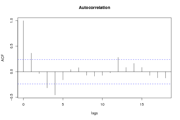
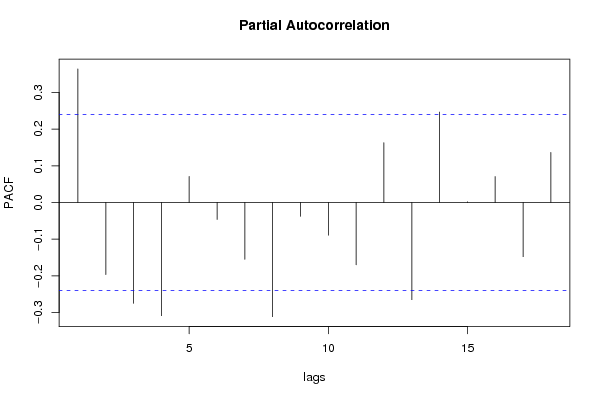
Title produced by software

(Partial) Autocorrelation Function

Date of computation

Fri, 12 Dec 2008 06:52:07 -0700

Cite this page as follows

Statistical Computations at FreeStatistics.org, Office for Research Development and Education, URL https://freestatistics.org/blog/index.php?v=date/2008/Dec/12/t122908997918kem2gnhg4ap60.htm/, Retrieved Sun, 19 May 2024 07:07:23 +0000

Statistical Computations at FreeStatistics.org, Office for Research Development and Education, URL https://freestatistics.org/blog/index.php?pk=32733, Retrieved Sun, 19 May 2024 07:07:23 +0000

QR Codes:

Paste this QR Code to cite your computation.

Original text written by user:

IsPrivate?

No (this computation is public)

User-defined keywords

Estimated Impact

159

Family? (F = Feedback message, R = changed R code, M = changed R Module, P = changed Parameters, D = changed Data)

-       [(Partial) Autocorrelation Function] [mannen pacf] [2008-12-12 13:52:07] [f24298b2e4c2a19d76cf4460ec5d2246] [Current]
-   PD    [(Partial) Autocorrelation Function] [pacf mannen meer ...] [2008-12-12 14:01:20] [e43247bc0ab243a5af99ac7f55ba0b41] 
-   P       [(Partial) Autocorrelation Function] [cor met lamda = 1 ] [2008-12-17 15:51:34] [e43247bc0ab243a5af99ac7f55ba0b41] 

Feedback Forum

Post a new message

Dataseries X:

Download CSV

Histogram

Boxplots

7,8
7,6
7,5
7,6
7,5
7,3
7,6
7,5
7,6
7,9
7,9
8,1
8,2
8,0
7,5
6,8
6,5
6,6
7,6
8,0
8,0
7,7
7,5
7,6
7,7
7,9
7,8
7,5
7,5
7,1
7,5
7,5
7,6
7,7
7,7
7,9
8,1
8,2
8,2
8,1
7,9
7,3
6,9
6,6
6,7
6,9
7,0
7,1
7,2
7,1
6,9
7,0
6,8
6,4
6,7
6,7
6,4
6,3
6,2
6,5
6,8
6,8
6,5
6,3
5,9
5,9
6,4
6,4

Summary of computational transaction
Raw Input	view raw input (R code)
Raw Output	view raw output of R engine
Computing time	1 seconds
R Server	'Gwilym Jenkins' @ 72.249.127.135

\begin{tabular}{lllllllll}
\hline
Summary of computational transaction \tabularnewline
Raw Input & view raw input (R code)  \tabularnewline
Raw Output & view raw output of R engine  \tabularnewline
Computing time & 1 seconds \tabularnewline
R Server & 'Gwilym Jenkins' @ 72.249.127.135 \tabularnewline
\hline
\end{tabular}
%Source: https://freestatistics.org/blog/index.php?pk=32733&T=0

[TABLE]
[ROW][C]Summary of computational transaction[/C][/ROW]
[ROW][C]Raw Input[/C][C]view raw input (R code) [/C][/ROW]
[ROW][C]Raw Output[/C][C]view raw output of R engine [/C][/ROW]
[ROW][C]Computing time[/C][C]1 seconds[/C][/ROW]
[ROW][C]R Server[/C][C]'Gwilym Jenkins' @ 72.249.127.135[/C][/ROW]
[/TABLE]
Source: https://freestatistics.org/blog/index.php?pk=32733&T=0

Globally Unique Identifier (entire table): ba.freestatistics.org/blog/index.php?pk=32733&T=0

As an alternative you can also use a QR Code:

The GUIDs for individual cells are displayed in the table below:

Summary of computational transaction
Raw Input	view raw input (R code)
Raw Output	view raw output of R engine
Computing time	1 seconds
R Server	'Gwilym Jenkins' @ 72.249.127.135

Autocorrelation Function
Time lag k	ACF(k)	T-STAT	P-value
1	0.364167	2.9808	0.002002
2	-0.037788	-0.3093	0.379025
3	-0.317456	-2.5985	0.005752
4	-0.456428	-3.736	0.000194
5	-0.160519	-1.3139	0.09668
6	0.043495	0.356	0.361472
7	0.080989	0.6629	0.254828
8	-0.070521	-0.5772	0.282856
9	-0.087354	-0.715	0.23854
10	-0.07238	-0.5925	0.277769
11	-0.022454	-0.1838	0.427365
12	0.282123	2.3093	0.01201
13	0.08453	0.6919	0.245694
14	0.163343	1.337	0.09287
15	0.084984	0.6956	0.244536
16	-0.073211	-0.5993	0.27551
17	-0.120281	-0.9845	0.164195
18	-0.124341	-1.0178	0.156224

\begin{tabular}{lllllllll}
\hline
Autocorrelation Function \tabularnewline
Time lag k & ACF(k) & T-STAT & P-value \tabularnewline
1 & 0.364167 & 2.9808 & 0.002002 \tabularnewline
2 & -0.037788 & -0.3093 & 0.379025 \tabularnewline
3 & -0.317456 & -2.5985 & 0.005752 \tabularnewline
4 & -0.456428 & -3.736 & 0.000194 \tabularnewline
5 & -0.160519 & -1.3139 & 0.09668 \tabularnewline
6 & 0.043495 & 0.356 & 0.361472 \tabularnewline
7 & 0.080989 & 0.6629 & 0.254828 \tabularnewline
8 & -0.070521 & -0.5772 & 0.282856 \tabularnewline
9 & -0.087354 & -0.715 & 0.23854 \tabularnewline
10 & -0.07238 & -0.5925 & 0.277769 \tabularnewline
11 & -0.022454 & -0.1838 & 0.427365 \tabularnewline
12 & 0.282123 & 2.3093 & 0.01201 \tabularnewline
13 & 0.08453 & 0.6919 & 0.245694 \tabularnewline
14 & 0.163343 & 1.337 & 0.09287 \tabularnewline
15 & 0.084984 & 0.6956 & 0.244536 \tabularnewline
16 & -0.073211 & -0.5993 & 0.27551 \tabularnewline
17 & -0.120281 & -0.9845 & 0.164195 \tabularnewline
18 & -0.124341 & -1.0178 & 0.156224 \tabularnewline
\hline
\end{tabular}
%Source: https://freestatistics.org/blog/index.php?pk=32733&T=1

[TABLE]
[ROW][C]Autocorrelation Function[/C][/ROW]
[ROW][C]Time lag k[/C][C]ACF(k)[/C][C]T-STAT[/C][C]P-value[/C][/ROW]
[ROW][C]1[/C][C]0.364167[/C][C]2.9808[/C][C]0.002002[/C][/ROW]
[ROW][C]2[/C][C]-0.037788[/C][C]-0.3093[/C][C]0.379025[/C][/ROW]
[ROW][C]3[/C][C]-0.317456[/C][C]-2.5985[/C][C]0.005752[/C][/ROW]
[ROW][C]4[/C][C]-0.456428[/C][C]-3.736[/C][C]0.000194[/C][/ROW]
[ROW][C]5[/C][C]-0.160519[/C][C]-1.3139[/C][C]0.09668[/C][/ROW]
[ROW][C]6[/C][C]0.043495[/C][C]0.356[/C][C]0.361472[/C][/ROW]
[ROW][C]7[/C][C]0.080989[/C][C]0.6629[/C][C]0.254828[/C][/ROW]
[ROW][C]8[/C][C]-0.070521[/C][C]-0.5772[/C][C]0.282856[/C][/ROW]
[ROW][C]9[/C][C]-0.087354[/C][C]-0.715[/C][C]0.23854[/C][/ROW]
[ROW][C]10[/C][C]-0.07238[/C][C]-0.5925[/C][C]0.277769[/C][/ROW]
[ROW][C]11[/C][C]-0.022454[/C][C]-0.1838[/C][C]0.427365[/C][/ROW]
[ROW][C]12[/C][C]0.282123[/C][C]2.3093[/C][C]0.01201[/C][/ROW]
[ROW][C]13[/C][C]0.08453[/C][C]0.6919[/C][C]0.245694[/C][/ROW]
[ROW][C]14[/C][C]0.163343[/C][C]1.337[/C][C]0.09287[/C][/ROW]
[ROW][C]15[/C][C]0.084984[/C][C]0.6956[/C][C]0.244536[/C][/ROW]
[ROW][C]16[/C][C]-0.073211[/C][C]-0.5993[/C][C]0.27551[/C][/ROW]
[ROW][C]17[/C][C]-0.120281[/C][C]-0.9845[/C][C]0.164195[/C][/ROW]
[ROW][C]18[/C][C]-0.124341[/C][C]-1.0178[/C][C]0.156224[/C][/ROW]
[/TABLE]
Source: https://freestatistics.org/blog/index.php?pk=32733&T=1

Globally Unique Identifier (entire table): ba.freestatistics.org/blog/index.php?pk=32733&T=1

As an alternative you can also use a QR Code:

The GUIDs for individual cells are displayed in the table below:

Autocorrelation Function
Time lag k	ACF(k)	T-STAT	P-value
1	0.364167	2.9808	0.002002
2	-0.037788	-0.3093	0.379025
3	-0.317456	-2.5985	0.005752
4	-0.456428	-3.736	0.000194
5	-0.160519	-1.3139	0.09668
6	0.043495	0.356	0.361472
7	0.080989	0.6629	0.254828
8	-0.070521	-0.5772	0.282856
9	-0.087354	-0.715	0.23854
10	-0.07238	-0.5925	0.277769
11	-0.022454	-0.1838	0.427365
12	0.282123	2.3093	0.01201
13	0.08453	0.6919	0.245694
14	0.163343	1.337	0.09287
15	0.084984	0.6956	0.244536
16	-0.073211	-0.5993	0.27551
17	-0.120281	-0.9845	0.164195
18	-0.124341	-1.0178	0.156224

Partial Autocorrelation Function
Time lag k	PACF(k)	T-STAT	P-value
1	0.364167	2.9808	0.002002
2	-0.19646	-1.6081	0.056259
3	-0.275148	-2.2522	0.013796
4	-0.308733	-2.5271	0.006934
5	0.071101	0.582	0.281265
6	-0.046161	-0.3778	0.353371
7	-0.155169	-1.2701	0.104219
8	-0.311396	-2.5489	0.006552
9	-0.037755	-0.309	0.379126
10	-0.089178	-0.73	0.233982
11	-0.170146	-1.3927	0.084157
12	0.163132	1.3353	0.09315
13	-0.265109	-2.17	0.016778
14	0.246627	2.0187	0.02376
15	0.001672	0.0137	0.494561
16	0.070838	0.5798	0.281987
17	-0.147709	-1.209	0.115447
18	0.13655	1.1177	0.133841

\begin{tabular}{lllllllll}
\hline
Partial Autocorrelation Function \tabularnewline
Time lag k & PACF(k) & T-STAT & P-value \tabularnewline
1 & 0.364167 & 2.9808 & 0.002002 \tabularnewline
2 & -0.19646 & -1.6081 & 0.056259 \tabularnewline
3 & -0.275148 & -2.2522 & 0.013796 \tabularnewline
4 & -0.308733 & -2.5271 & 0.006934 \tabularnewline
5 & 0.071101 & 0.582 & 0.281265 \tabularnewline
6 & -0.046161 & -0.3778 & 0.353371 \tabularnewline
7 & -0.155169 & -1.2701 & 0.104219 \tabularnewline
8 & -0.311396 & -2.5489 & 0.006552 \tabularnewline
9 & -0.037755 & -0.309 & 0.379126 \tabularnewline
10 & -0.089178 & -0.73 & 0.233982 \tabularnewline
11 & -0.170146 & -1.3927 & 0.084157 \tabularnewline
12 & 0.163132 & 1.3353 & 0.09315 \tabularnewline
13 & -0.265109 & -2.17 & 0.016778 \tabularnewline
14 & 0.246627 & 2.0187 & 0.02376 \tabularnewline
15 & 0.001672 & 0.0137 & 0.494561 \tabularnewline
16 & 0.070838 & 0.5798 & 0.281987 \tabularnewline
17 & -0.147709 & -1.209 & 0.115447 \tabularnewline
18 & 0.13655 & 1.1177 & 0.133841 \tabularnewline
\hline
\end{tabular}
%Source: https://freestatistics.org/blog/index.php?pk=32733&T=2

[TABLE]
[ROW][C]Partial Autocorrelation Function[/C][/ROW]
[ROW][C]Time lag k[/C][C]PACF(k)[/C][C]T-STAT[/C][C]P-value[/C][/ROW]
[ROW][C]1[/C][C]0.364167[/C][C]2.9808[/C][C]0.002002[/C][/ROW]
[ROW][C]2[/C][C]-0.19646[/C][C]-1.6081[/C][C]0.056259[/C][/ROW]
[ROW][C]3[/C][C]-0.275148[/C][C]-2.2522[/C][C]0.013796[/C][/ROW]
[ROW][C]4[/C][C]-0.308733[/C][C]-2.5271[/C][C]0.006934[/C][/ROW]
[ROW][C]5[/C][C]0.071101[/C][C]0.582[/C][C]0.281265[/C][/ROW]
[ROW][C]6[/C][C]-0.046161[/C][C]-0.3778[/C][C]0.353371[/C][/ROW]
[ROW][C]7[/C][C]-0.155169[/C][C]-1.2701[/C][C]0.104219[/C][/ROW]
[ROW][C]8[/C][C]-0.311396[/C][C]-2.5489[/C][C]0.006552[/C][/ROW]
[ROW][C]9[/C][C]-0.037755[/C][C]-0.309[/C][C]0.379126[/C][/ROW]
[ROW][C]10[/C][C]-0.089178[/C][C]-0.73[/C][C]0.233982[/C][/ROW]
[ROW][C]11[/C][C]-0.170146[/C][C]-1.3927[/C][C]0.084157[/C][/ROW]
[ROW][C]12[/C][C]0.163132[/C][C]1.3353[/C][C]0.09315[/C][/ROW]
[ROW][C]13[/C][C]-0.265109[/C][C]-2.17[/C][C]0.016778[/C][/ROW]
[ROW][C]14[/C][C]0.246627[/C][C]2.0187[/C][C]0.02376[/C][/ROW]
[ROW][C]15[/C][C]0.001672[/C][C]0.0137[/C][C]0.494561[/C][/ROW]
[ROW][C]16[/C][C]0.070838[/C][C]0.5798[/C][C]0.281987[/C][/ROW]
[ROW][C]17[/C][C]-0.147709[/C][C]-1.209[/C][C]0.115447[/C][/ROW]
[ROW][C]18[/C][C]0.13655[/C][C]1.1177[/C][C]0.133841[/C][/ROW]
[/TABLE]
Source: https://freestatistics.org/blog/index.php?pk=32733&T=2

Globally Unique Identifier (entire table): ba.freestatistics.org/blog/index.php?pk=32733&T=2

As an alternative you can also use a QR Code:

The GUIDs for individual cells are displayed in the table below:

Partial Autocorrelation Function
Time lag k	PACF(k)	T-STAT	P-value
1	0.364167	2.9808	0.002002
2	-0.19646	-1.6081	0.056259
3	-0.275148	-2.2522	0.013796
4	-0.308733	-2.5271	0.006934
5	0.071101	0.582	0.281265
6	-0.046161	-0.3778	0.353371
7	-0.155169	-1.2701	0.104219
8	-0.311396	-2.5489	0.006552
9	-0.037755	-0.309	0.379126
10	-0.089178	-0.73	0.233982
11	-0.170146	-1.3927	0.084157
12	0.163132	1.3353	0.09315
13	-0.265109	-2.17	0.016778
14	0.246627	2.0187	0.02376
15	0.001672	0.0137	0.494561
16	0.070838	0.5798	0.281987
17	-0.147709	-1.209	0.115447
18	0.13655	1.1177	0.133841

Figure 1

PNG link

Postscript link

PDF link

Figure 2

PNG link

Postscript link

PDF link

Parameters (Session):

par1 = Default ; par2 = 2.0 ; par3 = 1 ; par4 = 0 ; par5 = 12 ;

Parameters (R input):

par1 = Default ; par2 = 2.0 ; par3 = 1 ; par4 = 0 ; par5 = 12 ;

R code (references can be found in the software module):

if (par1 == 'Default') {
par1 = 10*log10(length(x))
} else {
par1 <- as.numeric(par1)
}
par2 <- as.numeric(par2)
par3 <- as.numeric(par3)
par4 <- as.numeric(par4)
par5 <- as.numeric(par5)
if (par2 == 0) {
x <- log(x)
} else {
x <- (x ^ par2 - 1) / par2
}
if (par3 > 0) x <- diff(x,lag=1,difference=par3)
if (par4 > 0) x <- diff(x,lag=par5,difference=par4)
bitmap(file='pic1.png')
racf <- acf(x,par1,main='Autocorrelation',xlab='lags',ylab='ACF')
dev.off()
bitmap(file='pic2.png')
rpacf <- pacf(x,par1,main='Partial Autocorrelation',xlab='lags',ylab='PACF')
dev.off()
(myacf <- c(racf$acf))
(mypacf <- c(rpacf$acf))
lengthx <- length(x)
sqrtn <- sqrt(lengthx)
load(file='createtable')
a<-table.start()
a<-table.row.start(a)
a<-table.element(a,'Autocorrelation Function',4,TRUE)
a<-table.row.end(a)
a<-table.row.start(a)
a<-table.element(a,'Time lag k',header=TRUE)
a<-table.element(a,hyperlink('basics.htm','ACF(k)','click here for more information about the Autocorrelation Function'),header=TRUE)
a<-table.element(a,'T-STAT',header=TRUE)
a<-table.element(a,'P-value',header=TRUE)
a<-table.row.end(a)
for (i in 2:(par1+1)) {
a<-table.row.start(a)
a<-table.element(a,i-1,header=TRUE)
a<-table.element(a,round(myacf[i],6))
mytstat <- myacf[i]*sqrtn
a<-table.element(a,round(mytstat,4))
a<-table.element(a,round(1-pt(abs(mytstat),lengthx),6))
a<-table.row.end(a)
}
a<-table.end(a)
table.save(a,file='mytable.tab')
a<-table.start()
a<-table.row.start(a)
a<-table.element(a,'Partial Autocorrelation Function',4,TRUE)
a<-table.row.end(a)
a<-table.row.start(a)
a<-table.element(a,'Time lag k',header=TRUE)
a<-table.element(a,hyperlink('basics.htm','PACF(k)','click here for more information about the Partial Autocorrelation Function'),header=TRUE)
a<-table.element(a,'T-STAT',header=TRUE)
a<-table.element(a,'P-value',header=TRUE)
a<-table.row.end(a)
for (i in 1:par1) {
a<-table.row.start(a)
a<-table.element(a,i,header=TRUE)
a<-table.element(a,round(mypacf[i],6))
mytstat <- mypacf[i]*sqrtn
a<-table.element(a,round(mytstat,4))
a<-table.element(a,round(1-pt(abs(mytstat),lengthx),6))
a<-table.row.end(a)
}
a<-table.end(a)
table.save(a,file='mytable1.tab')

Free Statistics

Description of Statistical Computation

Tree of Dependent Computations

Dataset

Tables (Output of Computation)

Figures (Output of Computation)

Input Parameters & R Code