Repository of Reproducible Computations

Free Statistics

of Irreproducible Research!

Author's title

Author

*The author of this computation has been verified*

R Software Module

rwasp_autocorrelation.wasp

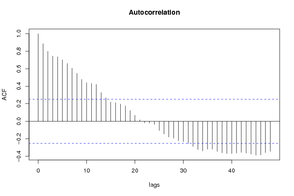
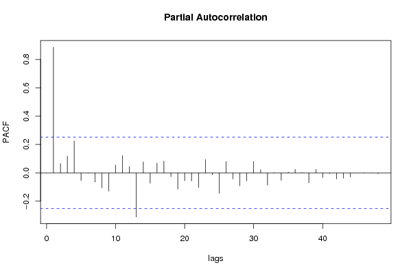
Title produced by software

(Partial) Autocorrelation Function

Date of computation

Fri, 12 Dec 2008 06:08:14 -0700

Cite this page as follows

Statistical Computations at FreeStatistics.org, Office for Research Development and Education, URL https://freestatistics.org/blog/index.php?v=date/2008/Dec/12/t1229087367zt423f42dz4h8hp.htm/, Retrieved Sun, 19 May 2024 03:57:29 +0000

Statistical Computations at FreeStatistics.org, Office for Research Development and Education, URL https://freestatistics.org/blog/index.php?pk=32668, Retrieved Sun, 19 May 2024 03:57:29 +0000

QR Codes:

Paste this QR Code to cite your computation.

Original text written by user:

IsPrivate?

No (this computation is public)

User-defined keywords

Estimated Impact

188

Family? (F = Feedback message, R = changed R code, M = changed R Module, P = changed Parameters, D = changed Data)

-     [Univariate Data Series] [Uitvoer.Nederland] [2008-12-03 15:11:10] [988ab43f527fc78aae41c84649095267]
-   P   [Univariate Data Series] [Export From Belgi...] [2008-12-03 15:52:29] [988ab43f527fc78aae41c84649095267]
- RMP     [(Partial) Autocorrelation Function] [Partial Autocorre...] [2008-12-03 16:01:07] [988ab43f527fc78aae41c84649095267]
-    D      [(Partial) Autocorrelation Function] [Partial Autocorre...] [2008-12-11 17:24:10] [988ab43f527fc78aae41c84649095267]
-   PD          [(Partial) Autocorrelation Function] [Partial Autocorre...] [2008-12-12 13:08:14] [5d823194959040fa9b19b8c8302177e6] [Current]
-                 [(Partial) Autocorrelation Function] [Partial Autocorre...] [2008-12-12 13:23:15] [988ab43f527fc78aae41c84649095267] 
-                 [(Partial) Autocorrelation Function] [Partial Autocorre...] [2008-12-12 13:25:37] [988ab43f527fc78aae41c84649095267] 

Feedback Forum

Post a new message

Dataseries X:

Download CSV

Histogram

Boxplots

Summary of computational transaction
Raw Input	view raw input (R code)
Raw Output	view raw output of R engine
Computing time	1 seconds
R Server	'Gwilym Jenkins' @ 72.249.127.135

\begin{tabular}{lllllllll}
\hline
Summary of computational transaction \tabularnewline
Raw Input & view raw input (R code)  \tabularnewline
Raw Output & view raw output of R engine  \tabularnewline
Computing time & 1 seconds \tabularnewline
R Server & 'Gwilym Jenkins' @ 72.249.127.135 \tabularnewline
\hline
\end{tabular}
%Source: https://freestatistics.org/blog/index.php?pk=32668&T=0

[TABLE]
[ROW][C]Summary of computational transaction[/C][/ROW]
[ROW][C]Raw Input[/C][C]view raw input (R code) [/C][/ROW]
[ROW][C]Raw Output[/C][C]view raw output of R engine [/C][/ROW]
[ROW][C]Computing time[/C][C]1 seconds[/C][/ROW]
[ROW][C]R Server[/C][C]'Gwilym Jenkins' @ 72.249.127.135[/C][/ROW]
[/TABLE]
Source: https://freestatistics.org/blog/index.php?pk=32668&T=0

Globally Unique Identifier (entire table): ba.freestatistics.org/blog/index.php?pk=32668&T=0

As an alternative you can also use a QR Code:

The GUIDs for individual cells are displayed in the table below:

Summary of computational transaction
Raw Input	view raw input (R code)
Raw Output	view raw output of R engine
Computing time	1 seconds
R Server	'Gwilym Jenkins' @ 72.249.127.135

Autocorrelation Function
Time lag k	ACF(k)	T-STAT	P-value
1	0.886322	6.8654	0
2	0.799572	6.1935	0
3	0.745328	5.7733	0
4	0.737731	5.7144	0
5	0.702483	5.4414	1e-06
6	0.661189	5.1215	2e-06
7	0.606516	4.6981	8e-06
8	0.548366	4.2476	3.8e-05
9	0.478121	3.7035	0.000232
10	0.440545	3.4124	0.000579
11	0.432173	3.3476	0.000706
12	0.421312	3.2635	0.00091
13	0.327787	2.539	0.006864
14	0.26864	2.0809	0.020861
15	0.219601	1.701	0.047058
16	0.212441	1.6456	0.052542
17	0.197261	1.528	0.065887
18	0.175431	1.3589	0.089636
19	0.121436	0.9406	0.175331
20	0.068098	0.5275	0.299901
21	0.016432	0.1273	0.449572
22	-0.01905	-0.1476	0.441591
23	-0.02166	-0.1678	0.433663
24	-0.036952	-0.2862	0.387844
25	-0.10635	-0.8238	0.206663
26	-0.145777	-1.1292	0.131658
27	-0.180794	-1.4004	0.083268
28	-0.194119	-1.5036	0.06896
29	-0.223486	-1.7311	0.044285
30	-0.234185	-1.814	0.03734
31	-0.255055	-1.9756	0.0264
32	-0.287539	-2.2273	0.014846
33	-0.32463	-2.5146	0.007308
34	-0.339663	-2.631	0.005402
35	-0.320395	-2.4818	0.007946
36	-0.320132	-2.4797	0.007987
37	-0.344937	-2.6719	0.004849
38	-0.361818	-2.8026	0.003408
39	-0.369967	-2.8658	0.002864
40	-0.368767	-2.8565	0.002939
41	-0.364363	-2.8223	0.003229
42	-0.356449	-2.761	0.003817
43	-0.365073	-2.8278	0.00318
44	-0.376285	-2.9147	0.002499
45	-0.387854	-3.0043	0.00194
46	-0.386012	-2.99	0.00202
47	-0.358687	-2.7784	0.003641
48	-0.344601	-2.6693	0.004882

\begin{tabular}{lllllllll}
\hline
Autocorrelation Function \tabularnewline
Time lag k & ACF(k) & T-STAT & P-value \tabularnewline
1 & 0.886322 & 6.8654 & 0 \tabularnewline
2 & 0.799572 & 6.1935 & 0 \tabularnewline
3 & 0.745328 & 5.7733 & 0 \tabularnewline
4 & 0.737731 & 5.7144 & 0 \tabularnewline
5 & 0.702483 & 5.4414 & 1e-06 \tabularnewline
6 & 0.661189 & 5.1215 & 2e-06 \tabularnewline
7 & 0.606516 & 4.6981 & 8e-06 \tabularnewline
8 & 0.548366 & 4.2476 & 3.8e-05 \tabularnewline
9 & 0.478121 & 3.7035 & 0.000232 \tabularnewline
10 & 0.440545 & 3.4124 & 0.000579 \tabularnewline
11 & 0.432173 & 3.3476 & 0.000706 \tabularnewline
12 & 0.421312 & 3.2635 & 0.00091 \tabularnewline
13 & 0.327787 & 2.539 & 0.006864 \tabularnewline
14 & 0.26864 & 2.0809 & 0.020861 \tabularnewline
15 & 0.219601 & 1.701 & 0.047058 \tabularnewline
16 & 0.212441 & 1.6456 & 0.052542 \tabularnewline
17 & 0.197261 & 1.528 & 0.065887 \tabularnewline
18 & 0.175431 & 1.3589 & 0.089636 \tabularnewline
19 & 0.121436 & 0.9406 & 0.175331 \tabularnewline
20 & 0.068098 & 0.5275 & 0.299901 \tabularnewline
21 & 0.016432 & 0.1273 & 0.449572 \tabularnewline
22 & -0.01905 & -0.1476 & 0.441591 \tabularnewline
23 & -0.02166 & -0.1678 & 0.433663 \tabularnewline
24 & -0.036952 & -0.2862 & 0.387844 \tabularnewline
25 & -0.10635 & -0.8238 & 0.206663 \tabularnewline
26 & -0.145777 & -1.1292 & 0.131658 \tabularnewline
27 & -0.180794 & -1.4004 & 0.083268 \tabularnewline
28 & -0.194119 & -1.5036 & 0.06896 \tabularnewline
29 & -0.223486 & -1.7311 & 0.044285 \tabularnewline
30 & -0.234185 & -1.814 & 0.03734 \tabularnewline
31 & -0.255055 & -1.9756 & 0.0264 \tabularnewline
32 & -0.287539 & -2.2273 & 0.014846 \tabularnewline
33 & -0.32463 & -2.5146 & 0.007308 \tabularnewline
34 & -0.339663 & -2.631 & 0.005402 \tabularnewline
35 & -0.320395 & -2.4818 & 0.007946 \tabularnewline
36 & -0.320132 & -2.4797 & 0.007987 \tabularnewline
37 & -0.344937 & -2.6719 & 0.004849 \tabularnewline
38 & -0.361818 & -2.8026 & 0.003408 \tabularnewline
39 & -0.369967 & -2.8658 & 0.002864 \tabularnewline
40 & -0.368767 & -2.8565 & 0.002939 \tabularnewline
41 & -0.364363 & -2.8223 & 0.003229 \tabularnewline
42 & -0.356449 & -2.761 & 0.003817 \tabularnewline
43 & -0.365073 & -2.8278 & 0.00318 \tabularnewline
44 & -0.376285 & -2.9147 & 0.002499 \tabularnewline
45 & -0.387854 & -3.0043 & 0.00194 \tabularnewline
46 & -0.386012 & -2.99 & 0.00202 \tabularnewline
47 & -0.358687 & -2.7784 & 0.003641 \tabularnewline
48 & -0.344601 & -2.6693 & 0.004882 \tabularnewline
\hline
\end{tabular}
%Source: https://freestatistics.org/blog/index.php?pk=32668&T=1

[TABLE]
[ROW][C]Autocorrelation Function[/C][/ROW]
[ROW][C]Time lag k[/C][C]ACF(k)[/C][C]T-STAT[/C][C]P-value[/C][/ROW]
[ROW][C]1[/C][C]0.886322[/C][C]6.8654[/C][C]0[/C][/ROW]
[ROW][C]2[/C][C]0.799572[/C][C]6.1935[/C][C]0[/C][/ROW]
[ROW][C]3[/C][C]0.745328[/C][C]5.7733[/C][C]0[/C][/ROW]
[ROW][C]4[/C][C]0.737731[/C][C]5.7144[/C][C]0[/C][/ROW]
[ROW][C]5[/C][C]0.702483[/C][C]5.4414[/C][C]1e-06[/C][/ROW]
[ROW][C]6[/C][C]0.661189[/C][C]5.1215[/C][C]2e-06[/C][/ROW]
[ROW][C]7[/C][C]0.606516[/C][C]4.6981[/C][C]8e-06[/C][/ROW]
[ROW][C]8[/C][C]0.548366[/C][C]4.2476[/C][C]3.8e-05[/C][/ROW]
[ROW][C]9[/C][C]0.478121[/C][C]3.7035[/C][C]0.000232[/C][/ROW]
[ROW][C]10[/C][C]0.440545[/C][C]3.4124[/C][C]0.000579[/C][/ROW]
[ROW][C]11[/C][C]0.432173[/C][C]3.3476[/C][C]0.000706[/C][/ROW]
[ROW][C]12[/C][C]0.421312[/C][C]3.2635[/C][C]0.00091[/C][/ROW]
[ROW][C]13[/C][C]0.327787[/C][C]2.539[/C][C]0.006864[/C][/ROW]
[ROW][C]14[/C][C]0.26864[/C][C]2.0809[/C][C]0.020861[/C][/ROW]
[ROW][C]15[/C][C]0.219601[/C][C]1.701[/C][C]0.047058[/C][/ROW]
[ROW][C]16[/C][C]0.212441[/C][C]1.6456[/C][C]0.052542[/C][/ROW]
[ROW][C]17[/C][C]0.197261[/C][C]1.528[/C][C]0.065887[/C][/ROW]
[ROW][C]18[/C][C]0.175431[/C][C]1.3589[/C][C]0.089636[/C][/ROW]
[ROW][C]19[/C][C]0.121436[/C][C]0.9406[/C][C]0.175331[/C][/ROW]
[ROW][C]20[/C][C]0.068098[/C][C]0.5275[/C][C]0.299901[/C][/ROW]
[ROW][C]21[/C][C]0.016432[/C][C]0.1273[/C][C]0.449572[/C][/ROW]
[ROW][C]22[/C][C]-0.01905[/C][C]-0.1476[/C][C]0.441591[/C][/ROW]
[ROW][C]23[/C][C]-0.02166[/C][C]-0.1678[/C][C]0.433663[/C][/ROW]
[ROW][C]24[/C][C]-0.036952[/C][C]-0.2862[/C][C]0.387844[/C][/ROW]
[ROW][C]25[/C][C]-0.10635[/C][C]-0.8238[/C][C]0.206663[/C][/ROW]
[ROW][C]26[/C][C]-0.145777[/C][C]-1.1292[/C][C]0.131658[/C][/ROW]
[ROW][C]27[/C][C]-0.180794[/C][C]-1.4004[/C][C]0.083268[/C][/ROW]
[ROW][C]28[/C][C]-0.194119[/C][C]-1.5036[/C][C]0.06896[/C][/ROW]
[ROW][C]29[/C][C]-0.223486[/C][C]-1.7311[/C][C]0.044285[/C][/ROW]
[ROW][C]30[/C][C]-0.234185[/C][C]-1.814[/C][C]0.03734[/C][/ROW]
[ROW][C]31[/C][C]-0.255055[/C][C]-1.9756[/C][C]0.0264[/C][/ROW]
[ROW][C]32[/C][C]-0.287539[/C][C]-2.2273[/C][C]0.014846[/C][/ROW]
[ROW][C]33[/C][C]-0.32463[/C][C]-2.5146[/C][C]0.007308[/C][/ROW]
[ROW][C]34[/C][C]-0.339663[/C][C]-2.631[/C][C]0.005402[/C][/ROW]
[ROW][C]35[/C][C]-0.320395[/C][C]-2.4818[/C][C]0.007946[/C][/ROW]
[ROW][C]36[/C][C]-0.320132[/C][C]-2.4797[/C][C]0.007987[/C][/ROW]
[ROW][C]37[/C][C]-0.344937[/C][C]-2.6719[/C][C]0.004849[/C][/ROW]
[ROW][C]38[/C][C]-0.361818[/C][C]-2.8026[/C][C]0.003408[/C][/ROW]
[ROW][C]39[/C][C]-0.369967[/C][C]-2.8658[/C][C]0.002864[/C][/ROW]
[ROW][C]40[/C][C]-0.368767[/C][C]-2.8565[/C][C]0.002939[/C][/ROW]
[ROW][C]41[/C][C]-0.364363[/C][C]-2.8223[/C][C]0.003229[/C][/ROW]
[ROW][C]42[/C][C]-0.356449[/C][C]-2.761[/C][C]0.003817[/C][/ROW]
[ROW][C]43[/C][C]-0.365073[/C][C]-2.8278[/C][C]0.00318[/C][/ROW]
[ROW][C]44[/C][C]-0.376285[/C][C]-2.9147[/C][C]0.002499[/C][/ROW]
[ROW][C]45[/C][C]-0.387854[/C][C]-3.0043[/C][C]0.00194[/C][/ROW]
[ROW][C]46[/C][C]-0.386012[/C][C]-2.99[/C][C]0.00202[/C][/ROW]
[ROW][C]47[/C][C]-0.358687[/C][C]-2.7784[/C][C]0.003641[/C][/ROW]
[ROW][C]48[/C][C]-0.344601[/C][C]-2.6693[/C][C]0.004882[/C][/ROW]
[/TABLE]
Source: https://freestatistics.org/blog/index.php?pk=32668&T=1

Globally Unique Identifier (entire table): ba.freestatistics.org/blog/index.php?pk=32668&T=1

As an alternative you can also use a QR Code:

The GUIDs for individual cells are displayed in the table below:

Autocorrelation Function
Time lag k	ACF(k)	T-STAT	P-value
1	0.886322	6.8654	0
2	0.799572	6.1935	0
3	0.745328	5.7733	0
4	0.737731	5.7144	0
5	0.702483	5.4414	1e-06
6	0.661189	5.1215	2e-06
7	0.606516	4.6981	8e-06
8	0.548366	4.2476	3.8e-05
9	0.478121	3.7035	0.000232
10	0.440545	3.4124	0.000579
11	0.432173	3.3476	0.000706
12	0.421312	3.2635	0.00091
13	0.327787	2.539	0.006864
14	0.26864	2.0809	0.020861
15	0.219601	1.701	0.047058
16	0.212441	1.6456	0.052542
17	0.197261	1.528	0.065887
18	0.175431	1.3589	0.089636
19	0.121436	0.9406	0.175331
20	0.068098	0.5275	0.299901
21	0.016432	0.1273	0.449572
22	-0.01905	-0.1476	0.441591
23	-0.02166	-0.1678	0.433663
24	-0.036952	-0.2862	0.387844
25	-0.10635	-0.8238	0.206663
26	-0.145777	-1.1292	0.131658
27	-0.180794	-1.4004	0.083268
28	-0.194119	-1.5036	0.06896
29	-0.223486	-1.7311	0.044285
30	-0.234185	-1.814	0.03734
31	-0.255055	-1.9756	0.0264
32	-0.287539	-2.2273	0.014846
33	-0.32463	-2.5146	0.007308
34	-0.339663	-2.631	0.005402
35	-0.320395	-2.4818	0.007946
36	-0.320132	-2.4797	0.007987
37	-0.344937	-2.6719	0.004849
38	-0.361818	-2.8026	0.003408
39	-0.369967	-2.8658	0.002864
40	-0.368767	-2.8565	0.002939
41	-0.364363	-2.8223	0.003229
42	-0.356449	-2.761	0.003817
43	-0.365073	-2.8278	0.00318
44	-0.376285	-2.9147	0.002499
45	-0.387854	-3.0043	0.00194
46	-0.386012	-2.99	0.00202
47	-0.358687	-2.7784	0.003641
48	-0.344601	-2.6693	0.004882

Partial Autocorrelation Function
Time lag k	PACF(k)	T-STAT	P-value
1	0.886322	6.8654	0
2	0.06531	0.5059	0.307394
3	0.117312	0.9087	0.183573
4	0.225544	1.7471	0.042872
5	-0.054014	-0.4184	0.338577
6	0.001582	0.0123	0.495133
7	-0.065017	-0.5036	0.308186
8	-0.105824	-0.8197	0.207813
9	-0.128825	-0.9979	0.161175
10	0.055228	0.4278	0.335167
11	0.122275	0.9471	0.173683
12	0.045358	0.3513	0.363281
13	-0.310702	-2.4067	0.009597
14	0.07706	0.5969	0.276409
15	-0.072588	-0.5623	0.288014
16	0.069112	0.5353	0.297197
17	0.082085	0.6358	0.263654
18	-0.026525	-0.2055	0.418952
19	-0.11416	-0.8843	0.190037
20	-0.055603	-0.4307	0.334115
21	-0.057121	-0.4425	0.329874
22	-0.102705	-0.7955	0.214716
23	0.093858	0.727	0.23502
24	-0.015104	-0.117	0.453628
25	-0.144755	-1.1213	0.13332
26	0.079912	0.619	0.269132
27	-0.042529	-0.3294	0.371489
28	-0.091103	-0.7057	0.241558
29	-0.056538	-0.4379	0.331501
30	0.080957	0.6271	0.266489
31	0.022665	0.1756	0.430616
32	-0.086697	-0.6716	0.252223
33	0.001884	0.0146	0.494204
34	-0.053228	-0.4123	0.340792
35	0.005039	0.039	0.484496
36	0.025327	0.1962	0.422565
37	0.003411	0.0264	0.489503
38	-0.071267	-0.552	0.291489
39	0.024365	0.1887	0.42547
40	-0.032867	-0.2546	0.399956
41	-0.004921	-0.0381	0.484861
42	-0.04341	-0.3363	0.368927
43	-0.037032	-0.2868	0.38761
44	-0.029989	-0.2323	0.408551
45	-0.000721	-0.0056	0.497783
46	0.001463	0.0113	0.495497
47	-0.000622	-0.0048	0.498087
48	-0.006056	-0.0469	0.481371

\begin{tabular}{lllllllll}
\hline
Partial Autocorrelation Function \tabularnewline
Time lag k & PACF(k) & T-STAT & P-value \tabularnewline
1 & 0.886322 & 6.8654 & 0 \tabularnewline
2 & 0.06531 & 0.5059 & 0.307394 \tabularnewline
3 & 0.117312 & 0.9087 & 0.183573 \tabularnewline
4 & 0.225544 & 1.7471 & 0.042872 \tabularnewline
5 & -0.054014 & -0.4184 & 0.338577 \tabularnewline
6 & 0.001582 & 0.0123 & 0.495133 \tabularnewline
7 & -0.065017 & -0.5036 & 0.308186 \tabularnewline
8 & -0.105824 & -0.8197 & 0.207813 \tabularnewline
9 & -0.128825 & -0.9979 & 0.161175 \tabularnewline
10 & 0.055228 & 0.4278 & 0.335167 \tabularnewline
11 & 0.122275 & 0.9471 & 0.173683 \tabularnewline
12 & 0.045358 & 0.3513 & 0.363281 \tabularnewline
13 & -0.310702 & -2.4067 & 0.009597 \tabularnewline
14 & 0.07706 & 0.5969 & 0.276409 \tabularnewline
15 & -0.072588 & -0.5623 & 0.288014 \tabularnewline
16 & 0.069112 & 0.5353 & 0.297197 \tabularnewline
17 & 0.082085 & 0.6358 & 0.263654 \tabularnewline
18 & -0.026525 & -0.2055 & 0.418952 \tabularnewline
19 & -0.11416 & -0.8843 & 0.190037 \tabularnewline
20 & -0.055603 & -0.4307 & 0.334115 \tabularnewline
21 & -0.057121 & -0.4425 & 0.329874 \tabularnewline
22 & -0.102705 & -0.7955 & 0.214716 \tabularnewline
23 & 0.093858 & 0.727 & 0.23502 \tabularnewline
24 & -0.015104 & -0.117 & 0.453628 \tabularnewline
25 & -0.144755 & -1.1213 & 0.13332 \tabularnewline
26 & 0.079912 & 0.619 & 0.269132 \tabularnewline
27 & -0.042529 & -0.3294 & 0.371489 \tabularnewline
28 & -0.091103 & -0.7057 & 0.241558 \tabularnewline
29 & -0.056538 & -0.4379 & 0.331501 \tabularnewline
30 & 0.080957 & 0.6271 & 0.266489 \tabularnewline
31 & 0.022665 & 0.1756 & 0.430616 \tabularnewline
32 & -0.086697 & -0.6716 & 0.252223 \tabularnewline
33 & 0.001884 & 0.0146 & 0.494204 \tabularnewline
34 & -0.053228 & -0.4123 & 0.340792 \tabularnewline
35 & 0.005039 & 0.039 & 0.484496 \tabularnewline
36 & 0.025327 & 0.1962 & 0.422565 \tabularnewline
37 & 0.003411 & 0.0264 & 0.489503 \tabularnewline
38 & -0.071267 & -0.552 & 0.291489 \tabularnewline
39 & 0.024365 & 0.1887 & 0.42547 \tabularnewline
40 & -0.032867 & -0.2546 & 0.399956 \tabularnewline
41 & -0.004921 & -0.0381 & 0.484861 \tabularnewline
42 & -0.04341 & -0.3363 & 0.368927 \tabularnewline
43 & -0.037032 & -0.2868 & 0.38761 \tabularnewline
44 & -0.029989 & -0.2323 & 0.408551 \tabularnewline
45 & -0.000721 & -0.0056 & 0.497783 \tabularnewline
46 & 0.001463 & 0.0113 & 0.495497 \tabularnewline
47 & -0.000622 & -0.0048 & 0.498087 \tabularnewline
48 & -0.006056 & -0.0469 & 0.481371 \tabularnewline
\hline
\end{tabular}
%Source: https://freestatistics.org/blog/index.php?pk=32668&T=2

[TABLE]
[ROW][C]Partial Autocorrelation Function[/C][/ROW]
[ROW][C]Time lag k[/C][C]PACF(k)[/C][C]T-STAT[/C][C]P-value[/C][/ROW]
[ROW][C]1[/C][C]0.886322[/C][C]6.8654[/C][C]0[/C][/ROW]
[ROW][C]2[/C][C]0.06531[/C][C]0.5059[/C][C]0.307394[/C][/ROW]
[ROW][C]3[/C][C]0.117312[/C][C]0.9087[/C][C]0.183573[/C][/ROW]
[ROW][C]4[/C][C]0.225544[/C][C]1.7471[/C][C]0.042872[/C][/ROW]
[ROW][C]5[/C][C]-0.054014[/C][C]-0.4184[/C][C]0.338577[/C][/ROW]
[ROW][C]6[/C][C]0.001582[/C][C]0.0123[/C][C]0.495133[/C][/ROW]
[ROW][C]7[/C][C]-0.065017[/C][C]-0.5036[/C][C]0.308186[/C][/ROW]
[ROW][C]8[/C][C]-0.105824[/C][C]-0.8197[/C][C]0.207813[/C][/ROW]
[ROW][C]9[/C][C]-0.128825[/C][C]-0.9979[/C][C]0.161175[/C][/ROW]
[ROW][C]10[/C][C]0.055228[/C][C]0.4278[/C][C]0.335167[/C][/ROW]
[ROW][C]11[/C][C]0.122275[/C][C]0.9471[/C][C]0.173683[/C][/ROW]
[ROW][C]12[/C][C]0.045358[/C][C]0.3513[/C][C]0.363281[/C][/ROW]
[ROW][C]13[/C][C]-0.310702[/C][C]-2.4067[/C][C]0.009597[/C][/ROW]
[ROW][C]14[/C][C]0.07706[/C][C]0.5969[/C][C]0.276409[/C][/ROW]
[ROW][C]15[/C][C]-0.072588[/C][C]-0.5623[/C][C]0.288014[/C][/ROW]
[ROW][C]16[/C][C]0.069112[/C][C]0.5353[/C][C]0.297197[/C][/ROW]
[ROW][C]17[/C][C]0.082085[/C][C]0.6358[/C][C]0.263654[/C][/ROW]
[ROW][C]18[/C][C]-0.026525[/C][C]-0.2055[/C][C]0.418952[/C][/ROW]
[ROW][C]19[/C][C]-0.11416[/C][C]-0.8843[/C][C]0.190037[/C][/ROW]
[ROW][C]20[/C][C]-0.055603[/C][C]-0.4307[/C][C]0.334115[/C][/ROW]
[ROW][C]21[/C][C]-0.057121[/C][C]-0.4425[/C][C]0.329874[/C][/ROW]
[ROW][C]22[/C][C]-0.102705[/C][C]-0.7955[/C][C]0.214716[/C][/ROW]
[ROW][C]23[/C][C]0.093858[/C][C]0.727[/C][C]0.23502[/C][/ROW]
[ROW][C]24[/C][C]-0.015104[/C][C]-0.117[/C][C]0.453628[/C][/ROW]
[ROW][C]25[/C][C]-0.144755[/C][C]-1.1213[/C][C]0.13332[/C][/ROW]
[ROW][C]26[/C][C]0.079912[/C][C]0.619[/C][C]0.269132[/C][/ROW]
[ROW][C]27[/C][C]-0.042529[/C][C]-0.3294[/C][C]0.371489[/C][/ROW]
[ROW][C]28[/C][C]-0.091103[/C][C]-0.7057[/C][C]0.241558[/C][/ROW]
[ROW][C]29[/C][C]-0.056538[/C][C]-0.4379[/C][C]0.331501[/C][/ROW]
[ROW][C]30[/C][C]0.080957[/C][C]0.6271[/C][C]0.266489[/C][/ROW]
[ROW][C]31[/C][C]0.022665[/C][C]0.1756[/C][C]0.430616[/C][/ROW]
[ROW][C]32[/C][C]-0.086697[/C][C]-0.6716[/C][C]0.252223[/C][/ROW]
[ROW][C]33[/C][C]0.001884[/C][C]0.0146[/C][C]0.494204[/C][/ROW]
[ROW][C]34[/C][C]-0.053228[/C][C]-0.4123[/C][C]0.340792[/C][/ROW]
[ROW][C]35[/C][C]0.005039[/C][C]0.039[/C][C]0.484496[/C][/ROW]
[ROW][C]36[/C][C]0.025327[/C][C]0.1962[/C][C]0.422565[/C][/ROW]
[ROW][C]37[/C][C]0.003411[/C][C]0.0264[/C][C]0.489503[/C][/ROW]
[ROW][C]38[/C][C]-0.071267[/C][C]-0.552[/C][C]0.291489[/C][/ROW]
[ROW][C]39[/C][C]0.024365[/C][C]0.1887[/C][C]0.42547[/C][/ROW]
[ROW][C]40[/C][C]-0.032867[/C][C]-0.2546[/C][C]0.399956[/C][/ROW]
[ROW][C]41[/C][C]-0.004921[/C][C]-0.0381[/C][C]0.484861[/C][/ROW]
[ROW][C]42[/C][C]-0.04341[/C][C]-0.3363[/C][C]0.368927[/C][/ROW]
[ROW][C]43[/C][C]-0.037032[/C][C]-0.2868[/C][C]0.38761[/C][/ROW]
[ROW][C]44[/C][C]-0.029989[/C][C]-0.2323[/C][C]0.408551[/C][/ROW]
[ROW][C]45[/C][C]-0.000721[/C][C]-0.0056[/C][C]0.497783[/C][/ROW]
[ROW][C]46[/C][C]0.001463[/C][C]0.0113[/C][C]0.495497[/C][/ROW]
[ROW][C]47[/C][C]-0.000622[/C][C]-0.0048[/C][C]0.498087[/C][/ROW]
[ROW][C]48[/C][C]-0.006056[/C][C]-0.0469[/C][C]0.481371[/C][/ROW]
[/TABLE]
Source: https://freestatistics.org/blog/index.php?pk=32668&T=2

Globally Unique Identifier (entire table): ba.freestatistics.org/blog/index.php?pk=32668&T=2

As an alternative you can also use a QR Code:

The GUIDs for individual cells are displayed in the table below:

Partial Autocorrelation Function
Time lag k	PACF(k)	T-STAT	P-value
1	0.886322	6.8654	0
2	0.06531	0.5059	0.307394
3	0.117312	0.9087	0.183573
4	0.225544	1.7471	0.042872
5	-0.054014	-0.4184	0.338577
6	0.001582	0.0123	0.495133
7	-0.065017	-0.5036	0.308186
8	-0.105824	-0.8197	0.207813
9	-0.128825	-0.9979	0.161175
10	0.055228	0.4278	0.335167
11	0.122275	0.9471	0.173683
12	0.045358	0.3513	0.363281
13	-0.310702	-2.4067	0.009597
14	0.07706	0.5969	0.276409
15	-0.072588	-0.5623	0.288014
16	0.069112	0.5353	0.297197
17	0.082085	0.6358	0.263654
18	-0.026525	-0.2055	0.418952
19	-0.11416	-0.8843	0.190037
20	-0.055603	-0.4307	0.334115
21	-0.057121	-0.4425	0.329874
22	-0.102705	-0.7955	0.214716
23	0.093858	0.727	0.23502
24	-0.015104	-0.117	0.453628
25	-0.144755	-1.1213	0.13332
26	0.079912	0.619	0.269132
27	-0.042529	-0.3294	0.371489
28	-0.091103	-0.7057	0.241558
29	-0.056538	-0.4379	0.331501
30	0.080957	0.6271	0.266489
31	0.022665	0.1756	0.430616
32	-0.086697	-0.6716	0.252223
33	0.001884	0.0146	0.494204
34	-0.053228	-0.4123	0.340792
35	0.005039	0.039	0.484496
36	0.025327	0.1962	0.422565
37	0.003411	0.0264	0.489503
38	-0.071267	-0.552	0.291489
39	0.024365	0.1887	0.42547
40	-0.032867	-0.2546	0.399956
41	-0.004921	-0.0381	0.484861
42	-0.04341	-0.3363	0.368927
43	-0.037032	-0.2868	0.38761
44	-0.029989	-0.2323	0.408551
45	-0.000721	-0.0056	0.497783
46	0.001463	0.0113	0.495497
47	-0.000622	-0.0048	0.498087
48	-0.006056	-0.0469	0.481371

Figure 1

PNG link

Postscript link

PDF link

Figure 2

PNG link

Postscript link

PDF link

Parameters (Session):

par1 = 12 ;

Parameters (R input):

par1 = 48 ; par2 = 0.1 ; par3 = 0 ; par4 = 0 ; par5 = 12 ;

R code (references can be found in the software module):

if (par1 == 'Default') {
par1 = 10*log10(length(x))
} else {
par1 <- as.numeric(par1)
}
par2 <- as.numeric(par2)
par3 <- as.numeric(par3)
par4 <- as.numeric(par4)
par5 <- as.numeric(par5)
if (par2 == 0) {
x <- log(x)
} else {
x <- (x ^ par2 - 1) / par2
}
if (par3 > 0) x <- diff(x,lag=1,difference=par3)
if (par4 > 0) x <- diff(x,lag=par5,difference=par4)
bitmap(file='pic1.png')
racf <- acf(x,par1,main='Autocorrelation',xlab='lags',ylab='ACF')
dev.off()
bitmap(file='pic2.png')
rpacf <- pacf(x,par1,main='Partial Autocorrelation',xlab='lags',ylab='PACF')
dev.off()
(myacf <- c(racf$acf))
(mypacf <- c(rpacf$acf))
lengthx <- length(x)
sqrtn <- sqrt(lengthx)
load(file='createtable')
a<-table.start()
a<-table.row.start(a)
a<-table.element(a,'Autocorrelation Function',4,TRUE)
a<-table.row.end(a)
a<-table.row.start(a)
a<-table.element(a,'Time lag k',header=TRUE)
a<-table.element(a,hyperlink('basics.htm','ACF(k)','click here for more information about the Autocorrelation Function'),header=TRUE)
a<-table.element(a,'T-STAT',header=TRUE)
a<-table.element(a,'P-value',header=TRUE)
a<-table.row.end(a)
for (i in 2:(par1+1)) {
a<-table.row.start(a)
a<-table.element(a,i-1,header=TRUE)
a<-table.element(a,round(myacf[i],6))
mytstat <- myacf[i]*sqrtn
a<-table.element(a,round(mytstat,4))
a<-table.element(a,round(1-pt(abs(mytstat),lengthx),6))
a<-table.row.end(a)
}
a<-table.end(a)
table.save(a,file='mytable.tab')
a<-table.start()
a<-table.row.start(a)
a<-table.element(a,'Partial Autocorrelation Function',4,TRUE)
a<-table.row.end(a)
a<-table.row.start(a)
a<-table.element(a,'Time lag k',header=TRUE)
a<-table.element(a,hyperlink('basics.htm','PACF(k)','click here for more information about the Partial Autocorrelation Function'),header=TRUE)
a<-table.element(a,'T-STAT',header=TRUE)
a<-table.element(a,'P-value',header=TRUE)
a<-table.row.end(a)
for (i in 1:par1) {
a<-table.row.start(a)
a<-table.element(a,i,header=TRUE)
a<-table.element(a,round(mypacf[i],6))
mytstat <- mypacf[i]*sqrtn
a<-table.element(a,round(mytstat,4))
a<-table.element(a,round(1-pt(abs(mytstat),lengthx),6))
a<-table.row.end(a)
}
a<-table.end(a)
table.save(a,file='mytable1.tab')

Free Statistics

Description of Statistical Computation

Tree of Dependent Computations

Dataset

Tables (Output of Computation)

Figures (Output of Computation)

Input Parameters & R Code