Free Statistics

of Irreproducible Research!

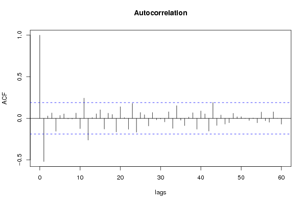
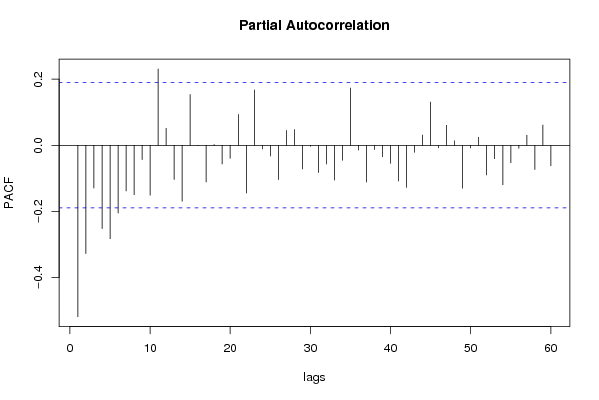
Author's title

(Partial) Autocorrelation voor het aantal faillissementen in het Vlaamse Ge...

Author

*The author of this computation has been verified*

R Software Module

rwasp_autocorrelation.wasp

Title produced by software

(Partial) Autocorrelation Function

Date of computation

Thu, 11 Dec 2008 08:23:01 -0700

Cite this page as follows

Statistical Computations at FreeStatistics.org, Office for Research Development and Education, URL https://freestatistics.org/blog/index.php?v=date/2008/Dec/11/t1229009020d68bgqamfoj5bjk.htm/, Retrieved Sun, 19 May 2024 07:24:21 +0000

Statistical Computations at FreeStatistics.org, Office for Research Development and Education, URL https://freestatistics.org/blog/index.php?pk=32309, Retrieved Sun, 19 May 2024 07:24:21 +0000

QR Codes:

Paste this QR Code to cite your computation.

Original text written by user:

IsPrivate?

No (this computation is public)

User-defined keywords

Estimated Impact

203

Family? (F = Feedback message, R = changed R code, M = changed R Module, P = changed Parameters, D = changed Data)

-     [(Partial) Autocorrelation Function] [(Partial) Autocor...] [2008-12-11 14:56:15] [87cabf13a90315c7085b765dcebb7412]
-   P   [(Partial) Autocorrelation Function] [(Partial) Autocor...] [2008-12-11 15:06:01] [87cabf13a90315c7085b765dcebb7412]
-   PD      [(Partial) Autocorrelation Function] [(Partial) Autocor...] [2008-12-11 15:23:01] [6fc58909ffe15c247a4f6748c8841ab4] [Current]
-   P         [(Partial) Autocorrelation Function] [(Partial) Autocor...] [2008-12-12 09:41:51] [87cabf13a90315c7085b765dcebb7412] 
-   P           [(Partial) Autocorrelation Function] [(Partial) Autocor...] [2008-12-12 09:46:16] [87cabf13a90315c7085b765dcebb7412] 
- RMPD          [Spectral Analysis] [Spectral Analysis...] [2008-12-12 09:54:07] [87cabf13a90315c7085b765dcebb7412] 
-   P             [Spectral Analysis] [Spectral Analysis...] [2008-12-12 10:06:12] [87cabf13a90315c7085b765dcebb7412] 
-   P               [Spectral Analysis] [Spectral Analysis...] [2008-12-12 10:11:50] [87cabf13a90315c7085b765dcebb7412] 
-   PD                [Spectral Analysis] [Spectral Analysis...] [2008-12-12 10:22:03] [87cabf13a90315c7085b765dcebb7412] 
-   P                   [Spectral Analysis] [Spectral Analysis...] [2008-12-12 10:29:35] [87cabf13a90315c7085b765dcebb7412] 
-    D          [(Partial) Autocorrelation Function] [autocorrelation < 20] [2008-12-18 14:35:59] [631938996a408f8d8cf3d9850ca0cd03] 
-   PD          [(Partial) Autocorrelation Function] [autocorrelation <...] [2008-12-18 14:42:48] [631938996a408f8d8cf3d9850ca0cd03] 
-   PD          [(Partial) Autocorrelation Function] [autocorrelation <...] [2008-12-18 14:46:54] [631938996a408f8d8cf3d9850ca0cd03] 
-   PD          [(Partial) Autocorrelation Function] [autocorrelation 2...] [2008-12-18 15:08:48] [631938996a408f8d8cf3d9850ca0cd03] 
-   PD          [(Partial) Autocorrelation Function] [autocorrelation 2...] [2008-12-18 15:13:35] [631938996a408f8d8cf3d9850ca0cd03] 
-                 [(Partial) Autocorrelation Function] [autocorrelation 2...] [2008-12-18 15:18:37] [631938996a408f8d8cf3d9850ca0cd03] 
- RM D            [Central Tendency] [central tendency ...] [2008-12-18 15:43:24] [631938996a408f8d8cf3d9850ca0cd03] 
-    D              [Central Tendency] [central tendency ...] [2008-12-18 15:52:59] [631938996a408f8d8cf3d9850ca0cd03] 
- RM                [Mean Plot] [mean plot tijdree...] [2008-12-18 16:03:30] [631938996a408f8d8cf3d9850ca0cd03] 
-    D                [Mean Plot] [mean plot tijdree...] [2008-12-18 16:10:04] [631938996a408f8d8cf3d9850ca0cd03] 

Feedback Forum

Post a new message

Dataseries X:

Download CSV

Histogram

Boxplots

Summary of computational transaction
Raw Input	view raw input (R code)
Raw Output	view raw output of R engine
Computing time	1 seconds
R Server	'George Udny Yule' @ 72.249.76.132

\begin{tabular}{lllllllll}
\hline
Summary of computational transaction \tabularnewline
Raw Input & view raw input (R code)  \tabularnewline
Raw Output & view raw output of R engine  \tabularnewline
Computing time & 1 seconds \tabularnewline
R Server & 'George Udny Yule' @ 72.249.76.132 \tabularnewline
\hline
\end{tabular}
%Source: https://freestatistics.org/blog/index.php?pk=32309&T=0

[TABLE]
[ROW][C]Summary of computational transaction[/C][/ROW]
[ROW][C]Raw Input[/C][C]view raw input (R code) [/C][/ROW]
[ROW][C]Raw Output[/C][C]view raw output of R engine [/C][/ROW]
[ROW][C]Computing time[/C][C]1 seconds[/C][/ROW]
[ROW][C]R Server[/C][C]'George Udny Yule' @ 72.249.76.132[/C][/ROW]
[/TABLE]
Source: https://freestatistics.org/blog/index.php?pk=32309&T=0

Globally Unique Identifier (entire table): ba.freestatistics.org/blog/index.php?pk=32309&T=0

As an alternative you can also use a QR Code:

The GUIDs for individual cells are displayed in the table below:

Summary of computational transaction
Raw Input	view raw input (R code)
Raw Output	view raw output of R engine
Computing time	1 seconds
R Server	'George Udny Yule' @ 72.249.76.132

Autocorrelation Function
Time lag k	ACF(k)	T-STAT	P-value
1	-0.518573	-5.3642	0
2	0.029348	0.3036	0.381018
3	0.065302	0.6755	0.25041
4	-0.154446	-1.5976	0.056541
5	0.035475	0.367	0.357189
6	0.053965	0.5582	0.28893
7	-0.006268	-0.0648	0.474213
8	-0.00666	-0.0689	0.472601
9	0.063545	0.6573	0.256196
10	-0.124061	-1.2833	0.101079
11	0.24335	2.5172	0.006655
12	-0.261152	-2.7014	0.004015
13	0.010072	0.1042	0.458608
14	0.054806	0.5669	0.28598
15	0.102674	1.0621	0.145297
16	-0.128732	-1.3316	0.092909
17	0.061938	0.6407	0.261545
18	0.04699	0.4861	0.313957
19	-0.16347	-1.6909	0.046879
20	0.139164	1.4395	0.07646
21	0.008105	0.0838	0.466673
22	-0.131009	-1.3552	0.089109
23	0.179767	1.8595	0.03285
24	-0.166057	-1.7177	0.044371
25	0.070228	0.7264	0.234576
26	0.04393	0.4544	0.325226
27	-0.091179	-0.9432	0.173861
28	0.070861	0.733	0.232584
29	-0.017794	-0.1841	0.427158
30	-0.006681	-0.0691	0.472515
31	-0.043072	-0.4455	0.328413
32	0.078859	0.8157	0.208234
33	-0.119992	-1.2412	0.108621
34	0.152166	1.574	0.059218
35	-0.021961	-0.2272	0.410363
36	-0.087649	-0.9066	0.183316
37	0.015014	0.1553	0.438436
38	0.067208	0.6952	0.244218
39	-0.130009	-1.3448	0.090763
40	0.088674	0.9173	0.180536
41	0.053497	0.5534	0.290581
42	-0.153559	-1.5884	0.05757
43	0.189975	1.9651	0.025996
44	-0.085367	-0.883	0.189597
45	0.04036	0.4175	0.338578
46	-0.069296	-0.7168	0.237528
47	-0.052881	-0.547	0.292755
48	0.060681	0.6277	0.265772
49	0.019011	0.1967	0.422237
50	0.019873	0.2056	0.418758
51	-0.001381	-0.0143	0.494316
52	-0.024982	-0.2584	0.398292
53	0.004725	0.0489	0.480554
54	-0.053877	-0.5573	0.289241
55	0.076201	0.7882	0.216153
56	-0.029459	-0.3047	0.380582
57	-0.046754	-0.4836	0.31482
58	0.078146	0.8083	0.210343
59	1.8e-05	2e-04	0.499925
60	-0.069551	-0.7194	0.23672

\begin{tabular}{lllllllll}
\hline
Autocorrelation Function \tabularnewline
Time lag k & ACF(k) & T-STAT & P-value \tabularnewline
1 & -0.518573 & -5.3642 & 0 \tabularnewline
2 & 0.029348 & 0.3036 & 0.381018 \tabularnewline
3 & 0.065302 & 0.6755 & 0.25041 \tabularnewline
4 & -0.154446 & -1.5976 & 0.056541 \tabularnewline
5 & 0.035475 & 0.367 & 0.357189 \tabularnewline
6 & 0.053965 & 0.5582 & 0.28893 \tabularnewline
7 & -0.006268 & -0.0648 & 0.474213 \tabularnewline
8 & -0.00666 & -0.0689 & 0.472601 \tabularnewline
9 & 0.063545 & 0.6573 & 0.256196 \tabularnewline
10 & -0.124061 & -1.2833 & 0.101079 \tabularnewline
11 & 0.24335 & 2.5172 & 0.006655 \tabularnewline
12 & -0.261152 & -2.7014 & 0.004015 \tabularnewline
13 & 0.010072 & 0.1042 & 0.458608 \tabularnewline
14 & 0.054806 & 0.5669 & 0.28598 \tabularnewline
15 & 0.102674 & 1.0621 & 0.145297 \tabularnewline
16 & -0.128732 & -1.3316 & 0.092909 \tabularnewline
17 & 0.061938 & 0.6407 & 0.261545 \tabularnewline
18 & 0.04699 & 0.4861 & 0.313957 \tabularnewline
19 & -0.16347 & -1.6909 & 0.046879 \tabularnewline
20 & 0.139164 & 1.4395 & 0.07646 \tabularnewline
21 & 0.008105 & 0.0838 & 0.466673 \tabularnewline
22 & -0.131009 & -1.3552 & 0.089109 \tabularnewline
23 & 0.179767 & 1.8595 & 0.03285 \tabularnewline
24 & -0.166057 & -1.7177 & 0.044371 \tabularnewline
25 & 0.070228 & 0.7264 & 0.234576 \tabularnewline
26 & 0.04393 & 0.4544 & 0.325226 \tabularnewline
27 & -0.091179 & -0.9432 & 0.173861 \tabularnewline
28 & 0.070861 & 0.733 & 0.232584 \tabularnewline
29 & -0.017794 & -0.1841 & 0.427158 \tabularnewline
30 & -0.006681 & -0.0691 & 0.472515 \tabularnewline
31 & -0.043072 & -0.4455 & 0.328413 \tabularnewline
32 & 0.078859 & 0.8157 & 0.208234 \tabularnewline
33 & -0.119992 & -1.2412 & 0.108621 \tabularnewline
34 & 0.152166 & 1.574 & 0.059218 \tabularnewline
35 & -0.021961 & -0.2272 & 0.410363 \tabularnewline
36 & -0.087649 & -0.9066 & 0.183316 \tabularnewline
37 & 0.015014 & 0.1553 & 0.438436 \tabularnewline
38 & 0.067208 & 0.6952 & 0.244218 \tabularnewline
39 & -0.130009 & -1.3448 & 0.090763 \tabularnewline
40 & 0.088674 & 0.9173 & 0.180536 \tabularnewline
41 & 0.053497 & 0.5534 & 0.290581 \tabularnewline
42 & -0.153559 & -1.5884 & 0.05757 \tabularnewline
43 & 0.189975 & 1.9651 & 0.025996 \tabularnewline
44 & -0.085367 & -0.883 & 0.189597 \tabularnewline
45 & 0.04036 & 0.4175 & 0.338578 \tabularnewline
46 & -0.069296 & -0.7168 & 0.237528 \tabularnewline
47 & -0.052881 & -0.547 & 0.292755 \tabularnewline
48 & 0.060681 & 0.6277 & 0.265772 \tabularnewline
49 & 0.019011 & 0.1967 & 0.422237 \tabularnewline
50 & 0.019873 & 0.2056 & 0.418758 \tabularnewline
51 & -0.001381 & -0.0143 & 0.494316 \tabularnewline
52 & -0.024982 & -0.2584 & 0.398292 \tabularnewline
53 & 0.004725 & 0.0489 & 0.480554 \tabularnewline
54 & -0.053877 & -0.5573 & 0.289241 \tabularnewline
55 & 0.076201 & 0.7882 & 0.216153 \tabularnewline
56 & -0.029459 & -0.3047 & 0.380582 \tabularnewline
57 & -0.046754 & -0.4836 & 0.31482 \tabularnewline
58 & 0.078146 & 0.8083 & 0.210343 \tabularnewline
59 & 1.8e-05 & 2e-04 & 0.499925 \tabularnewline
60 & -0.069551 & -0.7194 & 0.23672 \tabularnewline
\hline
\end{tabular}
%Source: https://freestatistics.org/blog/index.php?pk=32309&T=1

[TABLE]
[ROW][C]Autocorrelation Function[/C][/ROW]
[ROW][C]Time lag k[/C][C]ACF(k)[/C][C]T-STAT[/C][C]P-value[/C][/ROW]
[ROW][C]1[/C][C]-0.518573[/C][C]-5.3642[/C][C]0[/C][/ROW]
[ROW][C]2[/C][C]0.029348[/C][C]0.3036[/C][C]0.381018[/C][/ROW]
[ROW][C]3[/C][C]0.065302[/C][C]0.6755[/C][C]0.25041[/C][/ROW]
[ROW][C]4[/C][C]-0.154446[/C][C]-1.5976[/C][C]0.056541[/C][/ROW]
[ROW][C]5[/C][C]0.035475[/C][C]0.367[/C][C]0.357189[/C][/ROW]
[ROW][C]6[/C][C]0.053965[/C][C]0.5582[/C][C]0.28893[/C][/ROW]
[ROW][C]7[/C][C]-0.006268[/C][C]-0.0648[/C][C]0.474213[/C][/ROW]
[ROW][C]8[/C][C]-0.00666[/C][C]-0.0689[/C][C]0.472601[/C][/ROW]
[ROW][C]9[/C][C]0.063545[/C][C]0.6573[/C][C]0.256196[/C][/ROW]
[ROW][C]10[/C][C]-0.124061[/C][C]-1.2833[/C][C]0.101079[/C][/ROW]
[ROW][C]11[/C][C]0.24335[/C][C]2.5172[/C][C]0.006655[/C][/ROW]
[ROW][C]12[/C][C]-0.261152[/C][C]-2.7014[/C][C]0.004015[/C][/ROW]
[ROW][C]13[/C][C]0.010072[/C][C]0.1042[/C][C]0.458608[/C][/ROW]
[ROW][C]14[/C][C]0.054806[/C][C]0.5669[/C][C]0.28598[/C][/ROW]
[ROW][C]15[/C][C]0.102674[/C][C]1.0621[/C][C]0.145297[/C][/ROW]
[ROW][C]16[/C][C]-0.128732[/C][C]-1.3316[/C][C]0.092909[/C][/ROW]
[ROW][C]17[/C][C]0.061938[/C][C]0.6407[/C][C]0.261545[/C][/ROW]
[ROW][C]18[/C][C]0.04699[/C][C]0.4861[/C][C]0.313957[/C][/ROW]
[ROW][C]19[/C][C]-0.16347[/C][C]-1.6909[/C][C]0.046879[/C][/ROW]
[ROW][C]20[/C][C]0.139164[/C][C]1.4395[/C][C]0.07646[/C][/ROW]
[ROW][C]21[/C][C]0.008105[/C][C]0.0838[/C][C]0.466673[/C][/ROW]
[ROW][C]22[/C][C]-0.131009[/C][C]-1.3552[/C][C]0.089109[/C][/ROW]
[ROW][C]23[/C][C]0.179767[/C][C]1.8595[/C][C]0.03285[/C][/ROW]
[ROW][C]24[/C][C]-0.166057[/C][C]-1.7177[/C][C]0.044371[/C][/ROW]
[ROW][C]25[/C][C]0.070228[/C][C]0.7264[/C][C]0.234576[/C][/ROW]
[ROW][C]26[/C][C]0.04393[/C][C]0.4544[/C][C]0.325226[/C][/ROW]
[ROW][C]27[/C][C]-0.091179[/C][C]-0.9432[/C][C]0.173861[/C][/ROW]
[ROW][C]28[/C][C]0.070861[/C][C]0.733[/C][C]0.232584[/C][/ROW]
[ROW][C]29[/C][C]-0.017794[/C][C]-0.1841[/C][C]0.427158[/C][/ROW]
[ROW][C]30[/C][C]-0.006681[/C][C]-0.0691[/C][C]0.472515[/C][/ROW]
[ROW][C]31[/C][C]-0.043072[/C][C]-0.4455[/C][C]0.328413[/C][/ROW]
[ROW][C]32[/C][C]0.078859[/C][C]0.8157[/C][C]0.208234[/C][/ROW]
[ROW][C]33[/C][C]-0.119992[/C][C]-1.2412[/C][C]0.108621[/C][/ROW]
[ROW][C]34[/C][C]0.152166[/C][C]1.574[/C][C]0.059218[/C][/ROW]
[ROW][C]35[/C][C]-0.021961[/C][C]-0.2272[/C][C]0.410363[/C][/ROW]
[ROW][C]36[/C][C]-0.087649[/C][C]-0.9066[/C][C]0.183316[/C][/ROW]
[ROW][C]37[/C][C]0.015014[/C][C]0.1553[/C][C]0.438436[/C][/ROW]
[ROW][C]38[/C][C]0.067208[/C][C]0.6952[/C][C]0.244218[/C][/ROW]
[ROW][C]39[/C][C]-0.130009[/C][C]-1.3448[/C][C]0.090763[/C][/ROW]
[ROW][C]40[/C][C]0.088674[/C][C]0.9173[/C][C]0.180536[/C][/ROW]
[ROW][C]41[/C][C]0.053497[/C][C]0.5534[/C][C]0.290581[/C][/ROW]
[ROW][C]42[/C][C]-0.153559[/C][C]-1.5884[/C][C]0.05757[/C][/ROW]
[ROW][C]43[/C][C]0.189975[/C][C]1.9651[/C][C]0.025996[/C][/ROW]
[ROW][C]44[/C][C]-0.085367[/C][C]-0.883[/C][C]0.189597[/C][/ROW]
[ROW][C]45[/C][C]0.04036[/C][C]0.4175[/C][C]0.338578[/C][/ROW]
[ROW][C]46[/C][C]-0.069296[/C][C]-0.7168[/C][C]0.237528[/C][/ROW]
[ROW][C]47[/C][C]-0.052881[/C][C]-0.547[/C][C]0.292755[/C][/ROW]
[ROW][C]48[/C][C]0.060681[/C][C]0.6277[/C][C]0.265772[/C][/ROW]
[ROW][C]49[/C][C]0.019011[/C][C]0.1967[/C][C]0.422237[/C][/ROW]
[ROW][C]50[/C][C]0.019873[/C][C]0.2056[/C][C]0.418758[/C][/ROW]
[ROW][C]51[/C][C]-0.001381[/C][C]-0.0143[/C][C]0.494316[/C][/ROW]
[ROW][C]52[/C][C]-0.024982[/C][C]-0.2584[/C][C]0.398292[/C][/ROW]
[ROW][C]53[/C][C]0.004725[/C][C]0.0489[/C][C]0.480554[/C][/ROW]
[ROW][C]54[/C][C]-0.053877[/C][C]-0.5573[/C][C]0.289241[/C][/ROW]
[ROW][C]55[/C][C]0.076201[/C][C]0.7882[/C][C]0.216153[/C][/ROW]
[ROW][C]56[/C][C]-0.029459[/C][C]-0.3047[/C][C]0.380582[/C][/ROW]
[ROW][C]57[/C][C]-0.046754[/C][C]-0.4836[/C][C]0.31482[/C][/ROW]
[ROW][C]58[/C][C]0.078146[/C][C]0.8083[/C][C]0.210343[/C][/ROW]
[ROW][C]59[/C][C]1.8e-05[/C][C]2e-04[/C][C]0.499925[/C][/ROW]
[ROW][C]60[/C][C]-0.069551[/C][C]-0.7194[/C][C]0.23672[/C][/ROW]
[/TABLE]
Source: https://freestatistics.org/blog/index.php?pk=32309&T=1

Globally Unique Identifier (entire table): ba.freestatistics.org/blog/index.php?pk=32309&T=1

As an alternative you can also use a QR Code:

The GUIDs for individual cells are displayed in the table below:

Autocorrelation Function
Time lag k	ACF(k)	T-STAT	P-value
1	-0.518573	-5.3642	0
2	0.029348	0.3036	0.381018
3	0.065302	0.6755	0.25041
4	-0.154446	-1.5976	0.056541
5	0.035475	0.367	0.357189
6	0.053965	0.5582	0.28893
7	-0.006268	-0.0648	0.474213
8	-0.00666	-0.0689	0.472601
9	0.063545	0.6573	0.256196
10	-0.124061	-1.2833	0.101079
11	0.24335	2.5172	0.006655
12	-0.261152	-2.7014	0.004015
13	0.010072	0.1042	0.458608
14	0.054806	0.5669	0.28598
15	0.102674	1.0621	0.145297
16	-0.128732	-1.3316	0.092909
17	0.061938	0.6407	0.261545
18	0.04699	0.4861	0.313957
19	-0.16347	-1.6909	0.046879
20	0.139164	1.4395	0.07646
21	0.008105	0.0838	0.466673
22	-0.131009	-1.3552	0.089109
23	0.179767	1.8595	0.03285
24	-0.166057	-1.7177	0.044371
25	0.070228	0.7264	0.234576
26	0.04393	0.4544	0.325226
27	-0.091179	-0.9432	0.173861
28	0.070861	0.733	0.232584
29	-0.017794	-0.1841	0.427158
30	-0.006681	-0.0691	0.472515
31	-0.043072	-0.4455	0.328413
32	0.078859	0.8157	0.208234
33	-0.119992	-1.2412	0.108621
34	0.152166	1.574	0.059218
35	-0.021961	-0.2272	0.410363
36	-0.087649	-0.9066	0.183316
37	0.015014	0.1553	0.438436
38	0.067208	0.6952	0.244218
39	-0.130009	-1.3448	0.090763
40	0.088674	0.9173	0.180536
41	0.053497	0.5534	0.290581
42	-0.153559	-1.5884	0.05757
43	0.189975	1.9651	0.025996
44	-0.085367	-0.883	0.189597
45	0.04036	0.4175	0.338578
46	-0.069296	-0.7168	0.237528
47	-0.052881	-0.547	0.292755
48	0.060681	0.6277	0.265772
49	0.019011	0.1967	0.422237
50	0.019873	0.2056	0.418758
51	-0.001381	-0.0143	0.494316
52	-0.024982	-0.2584	0.398292
53	0.004725	0.0489	0.480554
54	-0.053877	-0.5573	0.289241
55	0.076201	0.7882	0.216153
56	-0.029459	-0.3047	0.380582
57	-0.046754	-0.4836	0.31482
58	0.078146	0.8083	0.210343
59	1.8e-05	2e-04	0.499925
60	-0.069551	-0.7194	0.23672

Partial Autocorrelation Function
Time lag k	PACF(k)	T-STAT	P-value
1	-0.518573	-5.3642	0
2	-0.327692	-3.3897	0.00049
3	-0.12937	-1.3382	0.091832
4	-0.251806	-2.6047	0.005251
5	-0.282467	-2.9219	0.002123
6	-0.204959	-2.1201	0.018154
7	-0.137962	-1.4271	0.078233
8	-0.149391	-1.5453	0.062612
9	-0.043294	-0.4478	0.327589
10	-0.151141	-1.5634	0.060454
11	0.23115	2.391	0.009274
12	0.051428	0.532	0.297924
13	-0.10316	-1.0671	0.144164
14	-0.16909	-1.7491	0.041572
15	0.153746	1.5904	0.057352
16	-0.000184	-0.0019	0.499244
17	-0.110897	-1.1471	0.126945
18	0.00221	0.0229	0.490902
19	-0.056201	-0.5814	0.281113
20	-0.039453	-0.4081	0.342007
21	0.093611	0.9683	0.167534
22	-0.144343	-1.4931	0.069177
23	0.167749	1.7352	0.042791
24	-0.01079	-0.1116	0.455672
25	-0.03218	-0.3329	0.369943
26	-0.103828	-1.074	0.142618
27	0.044924	0.4647	0.321545
28	0.047782	0.4943	0.311069
29	-0.071557	-0.7402	0.230404
30	-0.002882	-0.0298	0.488136
31	-0.082387	-0.8522	0.197999
32	-0.05623	-0.5817	0.281013
33	-0.105109	-1.0873	0.139684
34	-0.045291	-0.4685	0.320193
35	0.173365	1.7933	0.037875
36	-0.014303	-0.1479	0.441331
37	-0.111058	-1.1488	0.126602
38	-0.012931	-0.1338	0.446922
39	-0.034635	-0.3583	0.360425
40	-0.05455	-0.5643	0.286875
41	-0.108153	-1.1187	0.132878
42	-0.127684	-1.3208	0.094698
43	-0.021148	-0.2188	0.413628
44	0.031121	0.3219	0.37407
45	0.130944	1.3545	0.089216
46	-0.007529	-0.0779	0.469033
47	0.060735	0.6282	0.26559
48	0.013667	0.1414	0.443919
49	-0.129668	-1.3413	0.091331
50	-0.007844	-0.0811	0.467743
51	0.024517	0.2536	0.400145
52	-0.089763	-0.9285	0.177614
53	-0.040668	-0.4207	0.33742
54	-0.119491	-1.236	0.109578
55	-0.052599	-0.5441	0.293758
56	-0.009108	-0.0942	0.462558
57	0.030583	0.3164	0.376176
58	-0.073024	-0.7554	0.225845
59	0.061326	0.6344	0.263601
60	-0.061901	-0.6403	0.261671

\begin{tabular}{lllllllll}
\hline
Partial Autocorrelation Function \tabularnewline
Time lag k & PACF(k) & T-STAT & P-value \tabularnewline
1 & -0.518573 & -5.3642 & 0 \tabularnewline
2 & -0.327692 & -3.3897 & 0.00049 \tabularnewline
3 & -0.12937 & -1.3382 & 0.091832 \tabularnewline
4 & -0.251806 & -2.6047 & 0.005251 \tabularnewline
5 & -0.282467 & -2.9219 & 0.002123 \tabularnewline
6 & -0.204959 & -2.1201 & 0.018154 \tabularnewline
7 & -0.137962 & -1.4271 & 0.078233 \tabularnewline
8 & -0.149391 & -1.5453 & 0.062612 \tabularnewline
9 & -0.043294 & -0.4478 & 0.327589 \tabularnewline
10 & -0.151141 & -1.5634 & 0.060454 \tabularnewline
11 & 0.23115 & 2.391 & 0.009274 \tabularnewline
12 & 0.051428 & 0.532 & 0.297924 \tabularnewline
13 & -0.10316 & -1.0671 & 0.144164 \tabularnewline
14 & -0.16909 & -1.7491 & 0.041572 \tabularnewline
15 & 0.153746 & 1.5904 & 0.057352 \tabularnewline
16 & -0.000184 & -0.0019 & 0.499244 \tabularnewline
17 & -0.110897 & -1.1471 & 0.126945 \tabularnewline
18 & 0.00221 & 0.0229 & 0.490902 \tabularnewline
19 & -0.056201 & -0.5814 & 0.281113 \tabularnewline
20 & -0.039453 & -0.4081 & 0.342007 \tabularnewline
21 & 0.093611 & 0.9683 & 0.167534 \tabularnewline
22 & -0.144343 & -1.4931 & 0.069177 \tabularnewline
23 & 0.167749 & 1.7352 & 0.042791 \tabularnewline
24 & -0.01079 & -0.1116 & 0.455672 \tabularnewline
25 & -0.03218 & -0.3329 & 0.369943 \tabularnewline
26 & -0.103828 & -1.074 & 0.142618 \tabularnewline
27 & 0.044924 & 0.4647 & 0.321545 \tabularnewline
28 & 0.047782 & 0.4943 & 0.311069 \tabularnewline
29 & -0.071557 & -0.7402 & 0.230404 \tabularnewline
30 & -0.002882 & -0.0298 & 0.488136 \tabularnewline
31 & -0.082387 & -0.8522 & 0.197999 \tabularnewline
32 & -0.05623 & -0.5817 & 0.281013 \tabularnewline
33 & -0.105109 & -1.0873 & 0.139684 \tabularnewline
34 & -0.045291 & -0.4685 & 0.320193 \tabularnewline
35 & 0.173365 & 1.7933 & 0.037875 \tabularnewline
36 & -0.014303 & -0.1479 & 0.441331 \tabularnewline
37 & -0.111058 & -1.1488 & 0.126602 \tabularnewline
38 & -0.012931 & -0.1338 & 0.446922 \tabularnewline
39 & -0.034635 & -0.3583 & 0.360425 \tabularnewline
40 & -0.05455 & -0.5643 & 0.286875 \tabularnewline
41 & -0.108153 & -1.1187 & 0.132878 \tabularnewline
42 & -0.127684 & -1.3208 & 0.094698 \tabularnewline
43 & -0.021148 & -0.2188 & 0.413628 \tabularnewline
44 & 0.031121 & 0.3219 & 0.37407 \tabularnewline
45 & 0.130944 & 1.3545 & 0.089216 \tabularnewline
46 & -0.007529 & -0.0779 & 0.469033 \tabularnewline
47 & 0.060735 & 0.6282 & 0.26559 \tabularnewline
48 & 0.013667 & 0.1414 & 0.443919 \tabularnewline
49 & -0.129668 & -1.3413 & 0.091331 \tabularnewline
50 & -0.007844 & -0.0811 & 0.467743 \tabularnewline
51 & 0.024517 & 0.2536 & 0.400145 \tabularnewline
52 & -0.089763 & -0.9285 & 0.177614 \tabularnewline
53 & -0.040668 & -0.4207 & 0.33742 \tabularnewline
54 & -0.119491 & -1.236 & 0.109578 \tabularnewline
55 & -0.052599 & -0.5441 & 0.293758 \tabularnewline
56 & -0.009108 & -0.0942 & 0.462558 \tabularnewline
57 & 0.030583 & 0.3164 & 0.376176 \tabularnewline
58 & -0.073024 & -0.7554 & 0.225845 \tabularnewline
59 & 0.061326 & 0.6344 & 0.263601 \tabularnewline
60 & -0.061901 & -0.6403 & 0.261671 \tabularnewline
\hline
\end{tabular}
%Source: https://freestatistics.org/blog/index.php?pk=32309&T=2

[TABLE]
[ROW][C]Partial Autocorrelation Function[/C][/ROW]
[ROW][C]Time lag k[/C][C]PACF(k)[/C][C]T-STAT[/C][C]P-value[/C][/ROW]
[ROW][C]1[/C][C]-0.518573[/C][C]-5.3642[/C][C]0[/C][/ROW]
[ROW][C]2[/C][C]-0.327692[/C][C]-3.3897[/C][C]0.00049[/C][/ROW]
[ROW][C]3[/C][C]-0.12937[/C][C]-1.3382[/C][C]0.091832[/C][/ROW]
[ROW][C]4[/C][C]-0.251806[/C][C]-2.6047[/C][C]0.005251[/C][/ROW]
[ROW][C]5[/C][C]-0.282467[/C][C]-2.9219[/C][C]0.002123[/C][/ROW]
[ROW][C]6[/C][C]-0.204959[/C][C]-2.1201[/C][C]0.018154[/C][/ROW]
[ROW][C]7[/C][C]-0.137962[/C][C]-1.4271[/C][C]0.078233[/C][/ROW]
[ROW][C]8[/C][C]-0.149391[/C][C]-1.5453[/C][C]0.062612[/C][/ROW]
[ROW][C]9[/C][C]-0.043294[/C][C]-0.4478[/C][C]0.327589[/C][/ROW]
[ROW][C]10[/C][C]-0.151141[/C][C]-1.5634[/C][C]0.060454[/C][/ROW]
[ROW][C]11[/C][C]0.23115[/C][C]2.391[/C][C]0.009274[/C][/ROW]
[ROW][C]12[/C][C]0.051428[/C][C]0.532[/C][C]0.297924[/C][/ROW]
[ROW][C]13[/C][C]-0.10316[/C][C]-1.0671[/C][C]0.144164[/C][/ROW]
[ROW][C]14[/C][C]-0.16909[/C][C]-1.7491[/C][C]0.041572[/C][/ROW]
[ROW][C]15[/C][C]0.153746[/C][C]1.5904[/C][C]0.057352[/C][/ROW]
[ROW][C]16[/C][C]-0.000184[/C][C]-0.0019[/C][C]0.499244[/C][/ROW]
[ROW][C]17[/C][C]-0.110897[/C][C]-1.1471[/C][C]0.126945[/C][/ROW]
[ROW][C]18[/C][C]0.00221[/C][C]0.0229[/C][C]0.490902[/C][/ROW]
[ROW][C]19[/C][C]-0.056201[/C][C]-0.5814[/C][C]0.281113[/C][/ROW]
[ROW][C]20[/C][C]-0.039453[/C][C]-0.4081[/C][C]0.342007[/C][/ROW]
[ROW][C]21[/C][C]0.093611[/C][C]0.9683[/C][C]0.167534[/C][/ROW]
[ROW][C]22[/C][C]-0.144343[/C][C]-1.4931[/C][C]0.069177[/C][/ROW]
[ROW][C]23[/C][C]0.167749[/C][C]1.7352[/C][C]0.042791[/C][/ROW]
[ROW][C]24[/C][C]-0.01079[/C][C]-0.1116[/C][C]0.455672[/C][/ROW]
[ROW][C]25[/C][C]-0.03218[/C][C]-0.3329[/C][C]0.369943[/C][/ROW]
[ROW][C]26[/C][C]-0.103828[/C][C]-1.074[/C][C]0.142618[/C][/ROW]
[ROW][C]27[/C][C]0.044924[/C][C]0.4647[/C][C]0.321545[/C][/ROW]
[ROW][C]28[/C][C]0.047782[/C][C]0.4943[/C][C]0.311069[/C][/ROW]
[ROW][C]29[/C][C]-0.071557[/C][C]-0.7402[/C][C]0.230404[/C][/ROW]
[ROW][C]30[/C][C]-0.002882[/C][C]-0.0298[/C][C]0.488136[/C][/ROW]
[ROW][C]31[/C][C]-0.082387[/C][C]-0.8522[/C][C]0.197999[/C][/ROW]
[ROW][C]32[/C][C]-0.05623[/C][C]-0.5817[/C][C]0.281013[/C][/ROW]
[ROW][C]33[/C][C]-0.105109[/C][C]-1.0873[/C][C]0.139684[/C][/ROW]
[ROW][C]34[/C][C]-0.045291[/C][C]-0.4685[/C][C]0.320193[/C][/ROW]
[ROW][C]35[/C][C]0.173365[/C][C]1.7933[/C][C]0.037875[/C][/ROW]
[ROW][C]36[/C][C]-0.014303[/C][C]-0.1479[/C][C]0.441331[/C][/ROW]
[ROW][C]37[/C][C]-0.111058[/C][C]-1.1488[/C][C]0.126602[/C][/ROW]
[ROW][C]38[/C][C]-0.012931[/C][C]-0.1338[/C][C]0.446922[/C][/ROW]
[ROW][C]39[/C][C]-0.034635[/C][C]-0.3583[/C][C]0.360425[/C][/ROW]
[ROW][C]40[/C][C]-0.05455[/C][C]-0.5643[/C][C]0.286875[/C][/ROW]
[ROW][C]41[/C][C]-0.108153[/C][C]-1.1187[/C][C]0.132878[/C][/ROW]
[ROW][C]42[/C][C]-0.127684[/C][C]-1.3208[/C][C]0.094698[/C][/ROW]
[ROW][C]43[/C][C]-0.021148[/C][C]-0.2188[/C][C]0.413628[/C][/ROW]
[ROW][C]44[/C][C]0.031121[/C][C]0.3219[/C][C]0.37407[/C][/ROW]
[ROW][C]45[/C][C]0.130944[/C][C]1.3545[/C][C]0.089216[/C][/ROW]
[ROW][C]46[/C][C]-0.007529[/C][C]-0.0779[/C][C]0.469033[/C][/ROW]
[ROW][C]47[/C][C]0.060735[/C][C]0.6282[/C][C]0.26559[/C][/ROW]
[ROW][C]48[/C][C]0.013667[/C][C]0.1414[/C][C]0.443919[/C][/ROW]
[ROW][C]49[/C][C]-0.129668[/C][C]-1.3413[/C][C]0.091331[/C][/ROW]
[ROW][C]50[/C][C]-0.007844[/C][C]-0.0811[/C][C]0.467743[/C][/ROW]
[ROW][C]51[/C][C]0.024517[/C][C]0.2536[/C][C]0.400145[/C][/ROW]
[ROW][C]52[/C][C]-0.089763[/C][C]-0.9285[/C][C]0.177614[/C][/ROW]
[ROW][C]53[/C][C]-0.040668[/C][C]-0.4207[/C][C]0.33742[/C][/ROW]
[ROW][C]54[/C][C]-0.119491[/C][C]-1.236[/C][C]0.109578[/C][/ROW]
[ROW][C]55[/C][C]-0.052599[/C][C]-0.5441[/C][C]0.293758[/C][/ROW]
[ROW][C]56[/C][C]-0.009108[/C][C]-0.0942[/C][C]0.462558[/C][/ROW]
[ROW][C]57[/C][C]0.030583[/C][C]0.3164[/C][C]0.376176[/C][/ROW]
[ROW][C]58[/C][C]-0.073024[/C][C]-0.7554[/C][C]0.225845[/C][/ROW]
[ROW][C]59[/C][C]0.061326[/C][C]0.6344[/C][C]0.263601[/C][/ROW]
[ROW][C]60[/C][C]-0.061901[/C][C]-0.6403[/C][C]0.261671[/C][/ROW]
[/TABLE]
Source: https://freestatistics.org/blog/index.php?pk=32309&T=2

Globally Unique Identifier (entire table): ba.freestatistics.org/blog/index.php?pk=32309&T=2

As an alternative you can also use a QR Code:

The GUIDs for individual cells are displayed in the table below:

Partial Autocorrelation Function
Time lag k	PACF(k)	T-STAT	P-value
1	-0.518573	-5.3642	0
2	-0.327692	-3.3897	0.00049
3	-0.12937	-1.3382	0.091832
4	-0.251806	-2.6047	0.005251
5	-0.282467	-2.9219	0.002123
6	-0.204959	-2.1201	0.018154
7	-0.137962	-1.4271	0.078233
8	-0.149391	-1.5453	0.062612
9	-0.043294	-0.4478	0.327589
10	-0.151141	-1.5634	0.060454
11	0.23115	2.391	0.009274
12	0.051428	0.532	0.297924
13	-0.10316	-1.0671	0.144164
14	-0.16909	-1.7491	0.041572
15	0.153746	1.5904	0.057352
16	-0.000184	-0.0019	0.499244
17	-0.110897	-1.1471	0.126945
18	0.00221	0.0229	0.490902
19	-0.056201	-0.5814	0.281113
20	-0.039453	-0.4081	0.342007
21	0.093611	0.9683	0.167534
22	-0.144343	-1.4931	0.069177
23	0.167749	1.7352	0.042791
24	-0.01079	-0.1116	0.455672
25	-0.03218	-0.3329	0.369943
26	-0.103828	-1.074	0.142618
27	0.044924	0.4647	0.321545
28	0.047782	0.4943	0.311069
29	-0.071557	-0.7402	0.230404
30	-0.002882	-0.0298	0.488136
31	-0.082387	-0.8522	0.197999
32	-0.05623	-0.5817	0.281013
33	-0.105109	-1.0873	0.139684
34	-0.045291	-0.4685	0.320193
35	0.173365	1.7933	0.037875
36	-0.014303	-0.1479	0.441331
37	-0.111058	-1.1488	0.126602
38	-0.012931	-0.1338	0.446922
39	-0.034635	-0.3583	0.360425
40	-0.05455	-0.5643	0.286875
41	-0.108153	-1.1187	0.132878
42	-0.127684	-1.3208	0.094698
43	-0.021148	-0.2188	0.413628
44	0.031121	0.3219	0.37407
45	0.130944	1.3545	0.089216
46	-0.007529	-0.0779	0.469033
47	0.060735	0.6282	0.26559
48	0.013667	0.1414	0.443919
49	-0.129668	-1.3413	0.091331
50	-0.007844	-0.0811	0.467743
51	0.024517	0.2536	0.400145
52	-0.089763	-0.9285	0.177614
53	-0.040668	-0.4207	0.33742
54	-0.119491	-1.236	0.109578
55	-0.052599	-0.5441	0.293758
56	-0.009108	-0.0942	0.462558
57	0.030583	0.3164	0.376176
58	-0.073024	-0.7554	0.225845
59	0.061326	0.6344	0.263601
60	-0.061901	-0.6403	0.261671

Figure 1

PNG link

Postscript link

PDF link

Figure 2

PNG link

Postscript link

PDF link

Parameters (Session):

par1 = 60 ; par2 = 1 ; par3 = 1 ; par4 = 1 ; par5 = 12 ;

Parameters (R input):

par1 = 60 ; par2 = 1 ; par3 = 1 ; par4 = 1 ; par5 = 12 ;

R code (references can be found in the software module):

if (par1 == 'Default') {
par1 = 10*log10(length(x))
} else {
par1 <- as.numeric(par1)
}
par2 <- as.numeric(par2)
par3 <- as.numeric(par3)
par4 <- as.numeric(par4)
par5 <- as.numeric(par5)
if (par2 == 0) {
x <- log(x)
} else {
x <- (x ^ par2 - 1) / par2
}
if (par3 > 0) x <- diff(x,lag=1,difference=par3)
if (par4 > 0) x <- diff(x,lag=par5,difference=par4)
bitmap(file='pic1.png')
racf <- acf(x,par1,main='Autocorrelation',xlab='lags',ylab='ACF')
dev.off()
bitmap(file='pic2.png')
rpacf <- pacf(x,par1,main='Partial Autocorrelation',xlab='lags',ylab='PACF')
dev.off()
(myacf <- c(racf$acf))
(mypacf <- c(rpacf$acf))
lengthx <- length(x)
sqrtn <- sqrt(lengthx)
load(file='createtable')
a<-table.start()
a<-table.row.start(a)
a<-table.element(a,'Autocorrelation Function',4,TRUE)
a<-table.row.end(a)
a<-table.row.start(a)
a<-table.element(a,'Time lag k',header=TRUE)
a<-table.element(a,hyperlink('basics.htm','ACF(k)','click here for more information about the Autocorrelation Function'),header=TRUE)
a<-table.element(a,'T-STAT',header=TRUE)
a<-table.element(a,'P-value',header=TRUE)
a<-table.row.end(a)
for (i in 2:(par1+1)) {
a<-table.row.start(a)
a<-table.element(a,i-1,header=TRUE)
a<-table.element(a,round(myacf[i],6))
mytstat <- myacf[i]*sqrtn
a<-table.element(a,round(mytstat,4))
a<-table.element(a,round(1-pt(abs(mytstat),lengthx),6))
a<-table.row.end(a)
}
a<-table.end(a)
table.save(a,file='mytable.tab')
a<-table.start()
a<-table.row.start(a)
a<-table.element(a,'Partial Autocorrelation Function',4,TRUE)
a<-table.row.end(a)
a<-table.row.start(a)
a<-table.element(a,'Time lag k',header=TRUE)
a<-table.element(a,hyperlink('basics.htm','PACF(k)','click here for more information about the Partial Autocorrelation Function'),header=TRUE)
a<-table.element(a,'T-STAT',header=TRUE)
a<-table.element(a,'P-value',header=TRUE)
a<-table.row.end(a)
for (i in 1:par1) {
a<-table.row.start(a)
a<-table.element(a,i,header=TRUE)
a<-table.element(a,round(mypacf[i],6))
mytstat <- mypacf[i]*sqrtn
a<-table.element(a,round(mytstat,4))
a<-table.element(a,round(1-pt(abs(mytstat),lengthx),6))
a<-table.row.end(a)
}
a<-table.end(a)
table.save(a,file='mytable1.tab')

Free Statistics

Description of Statistical Computation

(Partial) Autocorrelation voor het aantal faillissementen in het Vlaamse Ge...

Tree of Dependent Computations

Dataset

Tables (Output of Computation)

Figures (Output of Computation)

Input Parameters & R Code