Repository of Reproducible Computations

Free Statistics

of Irreproducible Research!

Author's title

Author

*The author of this computation has been verified*

R Software Module

rwasp_autocorrelation.wasp

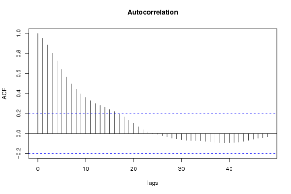
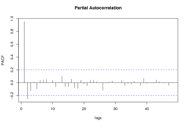
Title produced by software

(Partial) Autocorrelation Function

Date of computation

Wed, 10 Dec 2008 13:53:33 -0700

Cite this page as follows

Statistical Computations at FreeStatistics.org, Office for Research Development and Education, URL https://freestatistics.org/blog/index.php?v=date/2008/Dec/10/t1228942455mzeh935sqhrzce8.htm/, Retrieved Sun, 19 May 2024 05:34:41 +0000

Statistical Computations at FreeStatistics.org, Office for Research Development and Education, URL https://freestatistics.org/blog/index.php?pk=32112, Retrieved Sun, 19 May 2024 05:34:41 +0000

QR Codes:

Paste this QR Code to cite your computation.

Original text written by user:

IsPrivate?

No (this computation is public)

User-defined keywords

Estimated Impact

215

Family? (F = Feedback message, R = changed R code, M = changed R Module, P = changed Parameters, D = changed Data)

-       [(Partial) Autocorrelation Function] [tijdreeks - evolu...] [2008-12-10 20:53:33] [5a908f428dae694075b2a25ba39af7a8] [Current]

Feedback Forum

Post a new message

Dataseries X:

Download CSV

Histogram

Boxplots

Summary of computational transaction
Raw Input	view raw input (R code)
Raw Output	view raw output of R engine
Computing time	1 seconds
R Server	'George Udny Yule' @ 72.249.76.132

\begin{tabular}{lllllllll}
\hline
Summary of computational transaction \tabularnewline
Raw Input & view raw input (R code)  \tabularnewline
Raw Output & view raw output of R engine  \tabularnewline
Computing time & 1 seconds \tabularnewline
R Server & 'George Udny Yule' @ 72.249.76.132 \tabularnewline
\hline
\end{tabular}
%Source: https://freestatistics.org/blog/index.php?pk=32112&T=0

[TABLE]
[ROW][C]Summary of computational transaction[/C][/ROW]
[ROW][C]Raw Input[/C][C]view raw input (R code) [/C][/ROW]
[ROW][C]Raw Output[/C][C]view raw output of R engine [/C][/ROW]
[ROW][C]Computing time[/C][C]1 seconds[/C][/ROW]
[ROW][C]R Server[/C][C]'George Udny Yule' @ 72.249.76.132[/C][/ROW]
[/TABLE]
Source: https://freestatistics.org/blog/index.php?pk=32112&T=0

Globally Unique Identifier (entire table): ba.freestatistics.org/blog/index.php?pk=32112&T=0

As an alternative you can also use a QR Code:

The GUIDs for individual cells are displayed in the table below:

Summary of computational transaction
Raw Input	view raw input (R code)
Raw Output	view raw output of R engine
Computing time	1 seconds
R Server	'George Udny Yule' @ 72.249.76.132

Autocorrelation Function
Time lag k	ACF(k)	T-STAT	P-value
1	0.952907	9.3365	0
2	0.884781	8.669	0
3	0.804354	7.881	0
4	0.724825	7.1018	0
5	0.641002	6.2805	0
6	0.563864	5.5247	0
7	0.496226	4.862	2e-06
8	0.442197	4.3326	1.8e-05
9	0.396737	3.8872	9.3e-05
10	0.362001	3.5469	0.000302
11	0.328504	3.2187	0.000879
12	0.299334	2.9329	0.0021
13	0.280602	2.7493	0.003568
14	0.262727	2.5742	0.005788
15	0.240466	2.3561	0.010251
16	0.220879	2.1642	0.016466
17	0.197327	1.9334	0.028066
18	0.166348	1.6299	0.053203
19	0.134308	1.3159	0.095664
20	0.10215	1.0009	0.159704
21	0.068644	0.6726	0.251419
22	0.038206	0.3743	0.354488
23	0.016223	0.1589	0.437022
24	0.003233	0.0317	0.487397
25	-0.006203	-0.0608	0.475831
26	-0.020158	-0.1975	0.421924
27	-0.03288	-0.3222	0.374019
28	-0.046305	-0.4537	0.325537
29	-0.055098	-0.5398	0.295277
30	-0.061179	-0.5994	0.27515
31	-0.067361	-0.66	0.255418
32	-0.069947	-0.6853	0.247392
33	-0.071021	-0.6959	0.244099
34	-0.072842	-0.7137	0.23857
35	-0.0779	-0.7633	0.223589
36	-0.082482	-0.8082	0.2105
37	-0.0867	-0.8495	0.198862
38	-0.092447	-0.9058	0.183657
39	-0.093464	-0.9158	0.181044
40	-0.092643	-0.9077	0.183152
41	-0.089001	-0.872	0.192684
42	-0.085799	-0.8407	0.201314
43	-0.077968	-0.7639	0.223393
44	-0.067729	-0.6636	0.254267
45	-0.056911	-0.5576	0.289204
46	-0.047015	-0.4606	0.323046
47	-0.0401	-0.3929	0.347634
48	-0.035335	-0.3462	0.364971

\begin{tabular}{lllllllll}
\hline
Autocorrelation Function \tabularnewline
Time lag k & ACF(k) & T-STAT & P-value \tabularnewline
1 & 0.952907 & 9.3365 & 0 \tabularnewline
2 & 0.884781 & 8.669 & 0 \tabularnewline
3 & 0.804354 & 7.881 & 0 \tabularnewline
4 & 0.724825 & 7.1018 & 0 \tabularnewline
5 & 0.641002 & 6.2805 & 0 \tabularnewline
6 & 0.563864 & 5.5247 & 0 \tabularnewline
7 & 0.496226 & 4.862 & 2e-06 \tabularnewline
8 & 0.442197 & 4.3326 & 1.8e-05 \tabularnewline
9 & 0.396737 & 3.8872 & 9.3e-05 \tabularnewline
10 & 0.362001 & 3.5469 & 0.000302 \tabularnewline
11 & 0.328504 & 3.2187 & 0.000879 \tabularnewline
12 & 0.299334 & 2.9329 & 0.0021 \tabularnewline
13 & 0.280602 & 2.7493 & 0.003568 \tabularnewline
14 & 0.262727 & 2.5742 & 0.005788 \tabularnewline
15 & 0.240466 & 2.3561 & 0.010251 \tabularnewline
16 & 0.220879 & 2.1642 & 0.016466 \tabularnewline
17 & 0.197327 & 1.9334 & 0.028066 \tabularnewline
18 & 0.166348 & 1.6299 & 0.053203 \tabularnewline
19 & 0.134308 & 1.3159 & 0.095664 \tabularnewline
20 & 0.10215 & 1.0009 & 0.159704 \tabularnewline
21 & 0.068644 & 0.6726 & 0.251419 \tabularnewline
22 & 0.038206 & 0.3743 & 0.354488 \tabularnewline
23 & 0.016223 & 0.1589 & 0.437022 \tabularnewline
24 & 0.003233 & 0.0317 & 0.487397 \tabularnewline
25 & -0.006203 & -0.0608 & 0.475831 \tabularnewline
26 & -0.020158 & -0.1975 & 0.421924 \tabularnewline
27 & -0.03288 & -0.3222 & 0.374019 \tabularnewline
28 & -0.046305 & -0.4537 & 0.325537 \tabularnewline
29 & -0.055098 & -0.5398 & 0.295277 \tabularnewline
30 & -0.061179 & -0.5994 & 0.27515 \tabularnewline
31 & -0.067361 & -0.66 & 0.255418 \tabularnewline
32 & -0.069947 & -0.6853 & 0.247392 \tabularnewline
33 & -0.071021 & -0.6959 & 0.244099 \tabularnewline
34 & -0.072842 & -0.7137 & 0.23857 \tabularnewline
35 & -0.0779 & -0.7633 & 0.223589 \tabularnewline
36 & -0.082482 & -0.8082 & 0.2105 \tabularnewline
37 & -0.0867 & -0.8495 & 0.198862 \tabularnewline
38 & -0.092447 & -0.9058 & 0.183657 \tabularnewline
39 & -0.093464 & -0.9158 & 0.181044 \tabularnewline
40 & -0.092643 & -0.9077 & 0.183152 \tabularnewline
41 & -0.089001 & -0.872 & 0.192684 \tabularnewline
42 & -0.085799 & -0.8407 & 0.201314 \tabularnewline
43 & -0.077968 & -0.7639 & 0.223393 \tabularnewline
44 & -0.067729 & -0.6636 & 0.254267 \tabularnewline
45 & -0.056911 & -0.5576 & 0.289204 \tabularnewline
46 & -0.047015 & -0.4606 & 0.323046 \tabularnewline
47 & -0.0401 & -0.3929 & 0.347634 \tabularnewline
48 & -0.035335 & -0.3462 & 0.364971 \tabularnewline
\hline
\end{tabular}
%Source: https://freestatistics.org/blog/index.php?pk=32112&T=1

[TABLE]
[ROW][C]Autocorrelation Function[/C][/ROW]
[ROW][C]Time lag k[/C][C]ACF(k)[/C][C]T-STAT[/C][C]P-value[/C][/ROW]
[ROW][C]1[/C][C]0.952907[/C][C]9.3365[/C][C]0[/C][/ROW]
[ROW][C]2[/C][C]0.884781[/C][C]8.669[/C][C]0[/C][/ROW]
[ROW][C]3[/C][C]0.804354[/C][C]7.881[/C][C]0[/C][/ROW]
[ROW][C]4[/C][C]0.724825[/C][C]7.1018[/C][C]0[/C][/ROW]
[ROW][C]5[/C][C]0.641002[/C][C]6.2805[/C][C]0[/C][/ROW]
[ROW][C]6[/C][C]0.563864[/C][C]5.5247[/C][C]0[/C][/ROW]
[ROW][C]7[/C][C]0.496226[/C][C]4.862[/C][C]2e-06[/C][/ROW]
[ROW][C]8[/C][C]0.442197[/C][C]4.3326[/C][C]1.8e-05[/C][/ROW]
[ROW][C]9[/C][C]0.396737[/C][C]3.8872[/C][C]9.3e-05[/C][/ROW]
[ROW][C]10[/C][C]0.362001[/C][C]3.5469[/C][C]0.000302[/C][/ROW]
[ROW][C]11[/C][C]0.328504[/C][C]3.2187[/C][C]0.000879[/C][/ROW]
[ROW][C]12[/C][C]0.299334[/C][C]2.9329[/C][C]0.0021[/C][/ROW]
[ROW][C]13[/C][C]0.280602[/C][C]2.7493[/C][C]0.003568[/C][/ROW]
[ROW][C]14[/C][C]0.262727[/C][C]2.5742[/C][C]0.005788[/C][/ROW]
[ROW][C]15[/C][C]0.240466[/C][C]2.3561[/C][C]0.010251[/C][/ROW]
[ROW][C]16[/C][C]0.220879[/C][C]2.1642[/C][C]0.016466[/C][/ROW]
[ROW][C]17[/C][C]0.197327[/C][C]1.9334[/C][C]0.028066[/C][/ROW]
[ROW][C]18[/C][C]0.166348[/C][C]1.6299[/C][C]0.053203[/C][/ROW]
[ROW][C]19[/C][C]0.134308[/C][C]1.3159[/C][C]0.095664[/C][/ROW]
[ROW][C]20[/C][C]0.10215[/C][C]1.0009[/C][C]0.159704[/C][/ROW]
[ROW][C]21[/C][C]0.068644[/C][C]0.6726[/C][C]0.251419[/C][/ROW]
[ROW][C]22[/C][C]0.038206[/C][C]0.3743[/C][C]0.354488[/C][/ROW]
[ROW][C]23[/C][C]0.016223[/C][C]0.1589[/C][C]0.437022[/C][/ROW]
[ROW][C]24[/C][C]0.003233[/C][C]0.0317[/C][C]0.487397[/C][/ROW]
[ROW][C]25[/C][C]-0.006203[/C][C]-0.0608[/C][C]0.475831[/C][/ROW]
[ROW][C]26[/C][C]-0.020158[/C][C]-0.1975[/C][C]0.421924[/C][/ROW]
[ROW][C]27[/C][C]-0.03288[/C][C]-0.3222[/C][C]0.374019[/C][/ROW]
[ROW][C]28[/C][C]-0.046305[/C][C]-0.4537[/C][C]0.325537[/C][/ROW]
[ROW][C]29[/C][C]-0.055098[/C][C]-0.5398[/C][C]0.295277[/C][/ROW]
[ROW][C]30[/C][C]-0.061179[/C][C]-0.5994[/C][C]0.27515[/C][/ROW]
[ROW][C]31[/C][C]-0.067361[/C][C]-0.66[/C][C]0.255418[/C][/ROW]
[ROW][C]32[/C][C]-0.069947[/C][C]-0.6853[/C][C]0.247392[/C][/ROW]
[ROW][C]33[/C][C]-0.071021[/C][C]-0.6959[/C][C]0.244099[/C][/ROW]
[ROW][C]34[/C][C]-0.072842[/C][C]-0.7137[/C][C]0.23857[/C][/ROW]
[ROW][C]35[/C][C]-0.0779[/C][C]-0.7633[/C][C]0.223589[/C][/ROW]
[ROW][C]36[/C][C]-0.082482[/C][C]-0.8082[/C][C]0.2105[/C][/ROW]
[ROW][C]37[/C][C]-0.0867[/C][C]-0.8495[/C][C]0.198862[/C][/ROW]
[ROW][C]38[/C][C]-0.092447[/C][C]-0.9058[/C][C]0.183657[/C][/ROW]
[ROW][C]39[/C][C]-0.093464[/C][C]-0.9158[/C][C]0.181044[/C][/ROW]
[ROW][C]40[/C][C]-0.092643[/C][C]-0.9077[/C][C]0.183152[/C][/ROW]
[ROW][C]41[/C][C]-0.089001[/C][C]-0.872[/C][C]0.192684[/C][/ROW]
[ROW][C]42[/C][C]-0.085799[/C][C]-0.8407[/C][C]0.201314[/C][/ROW]
[ROW][C]43[/C][C]-0.077968[/C][C]-0.7639[/C][C]0.223393[/C][/ROW]
[ROW][C]44[/C][C]-0.067729[/C][C]-0.6636[/C][C]0.254267[/C][/ROW]
[ROW][C]45[/C][C]-0.056911[/C][C]-0.5576[/C][C]0.289204[/C][/ROW]
[ROW][C]46[/C][C]-0.047015[/C][C]-0.4606[/C][C]0.323046[/C][/ROW]
[ROW][C]47[/C][C]-0.0401[/C][C]-0.3929[/C][C]0.347634[/C][/ROW]
[ROW][C]48[/C][C]-0.035335[/C][C]-0.3462[/C][C]0.364971[/C][/ROW]
[/TABLE]
Source: https://freestatistics.org/blog/index.php?pk=32112&T=1

Globally Unique Identifier (entire table): ba.freestatistics.org/blog/index.php?pk=32112&T=1

As an alternative you can also use a QR Code:

The GUIDs for individual cells are displayed in the table below:

Autocorrelation Function
Time lag k	ACF(k)	T-STAT	P-value
1	0.952907	9.3365	0
2	0.884781	8.669	0
3	0.804354	7.881	0
4	0.724825	7.1018	0
5	0.641002	6.2805	0
6	0.563864	5.5247	0
7	0.496226	4.862	2e-06
8	0.442197	4.3326	1.8e-05
9	0.396737	3.8872	9.3e-05
10	0.362001	3.5469	0.000302
11	0.328504	3.2187	0.000879
12	0.299334	2.9329	0.0021
13	0.280602	2.7493	0.003568
14	0.262727	2.5742	0.005788
15	0.240466	2.3561	0.010251
16	0.220879	2.1642	0.016466
17	0.197327	1.9334	0.028066
18	0.166348	1.6299	0.053203
19	0.134308	1.3159	0.095664
20	0.10215	1.0009	0.159704
21	0.068644	0.6726	0.251419
22	0.038206	0.3743	0.354488
23	0.016223	0.1589	0.437022
24	0.003233	0.0317	0.487397
25	-0.006203	-0.0608	0.475831
26	-0.020158	-0.1975	0.421924
27	-0.03288	-0.3222	0.374019
28	-0.046305	-0.4537	0.325537
29	-0.055098	-0.5398	0.295277
30	-0.061179	-0.5994	0.27515
31	-0.067361	-0.66	0.255418
32	-0.069947	-0.6853	0.247392
33	-0.071021	-0.6959	0.244099
34	-0.072842	-0.7137	0.23857
35	-0.0779	-0.7633	0.223589
36	-0.082482	-0.8082	0.2105
37	-0.0867	-0.8495	0.198862
38	-0.092447	-0.9058	0.183657
39	-0.093464	-0.9158	0.181044
40	-0.092643	-0.9077	0.183152
41	-0.089001	-0.872	0.192684
42	-0.085799	-0.8407	0.201314
43	-0.077968	-0.7639	0.223393
44	-0.067729	-0.6636	0.254267
45	-0.056911	-0.5576	0.289204
46	-0.047015	-0.4606	0.323046
47	-0.0401	-0.3929	0.347634
48	-0.035335	-0.3462	0.364971

Partial Autocorrelation Function
Time lag k	PACF(k)	T-STAT	P-value
1	0.952907	9.3365	0
2	-0.252822	-2.4771	0.007496
3	-0.127806	-1.2522	0.106763
4	0.012288	0.1204	0.452209
5	-0.099073	-0.9707	0.167066
6	0.038992	0.382	0.351636
7	0.042658	0.418	0.338454
8	0.054769	0.5366	0.296384
9	0.000911	0.0089	0.496448
10	0.03787	0.371	0.355711
11	-0.064683	-0.6338	0.263871
12	0.005668	0.0555	0.477913
13	0.10307	1.0099	0.157548
14	-0.060082	-0.5887	0.278727
15	-0.061291	-0.6005	0.274786
16	0.058172	0.57	0.285016
17	-0.080932	-0.793	0.214877
18	-0.090915	-0.8908	0.187637
19	0.042923	0.4206	0.337508
20	-0.022463	-0.2201	0.413134
21	-0.048096	-0.4712	0.319269
22	0.043346	0.4247	0.336003
23	0.039189	0.384	0.350925
24	0.016128	0.158	0.437386
25	-0.000722	-0.0071	0.497186
26	-0.118907	-1.165	0.123443
27	-0.006175	-0.0605	0.47594
28	0.013247	0.1298	0.448502
29	0.027387	0.2683	0.394508
30	0.003646	0.0357	0.485789
31	0.000652	0.0064	0.497457
32	0.03378	0.331	0.370691
33	-0.046244	-0.4531	0.32575
34	-0.013622	-0.1335	0.44705
35	-0.023261	-0.2279	0.4101
36	0.02082	0.204	0.419394
37	0.00195	0.0191	0.492396
38	-0.043027	-0.4216	0.337139
39	0.067917	0.6654	0.25368
40	-0.016882	-0.1654	0.434486
41	-0.003783	-0.0371	0.485254
42	-0.008929	-0.0875	0.465234
43	0.046116	0.4518	0.326199
44	0.019129	0.1874	0.425861
45	-0.0039	-0.0382	0.484798
46	-0.001379	-0.0135	0.494625
47	-0.041413	-0.4058	0.342912
48	0.002496	0.0245	0.490269

\begin{tabular}{lllllllll}
\hline
Partial Autocorrelation Function \tabularnewline
Time lag k & PACF(k) & T-STAT & P-value \tabularnewline
1 & 0.952907 & 9.3365 & 0 \tabularnewline
2 & -0.252822 & -2.4771 & 0.007496 \tabularnewline
3 & -0.127806 & -1.2522 & 0.106763 \tabularnewline
4 & 0.012288 & 0.1204 & 0.452209 \tabularnewline
5 & -0.099073 & -0.9707 & 0.167066 \tabularnewline
6 & 0.038992 & 0.382 & 0.351636 \tabularnewline
7 & 0.042658 & 0.418 & 0.338454 \tabularnewline
8 & 0.054769 & 0.5366 & 0.296384 \tabularnewline
9 & 0.000911 & 0.0089 & 0.496448 \tabularnewline
10 & 0.03787 & 0.371 & 0.355711 \tabularnewline
11 & -0.064683 & -0.6338 & 0.263871 \tabularnewline
12 & 0.005668 & 0.0555 & 0.477913 \tabularnewline
13 & 0.10307 & 1.0099 & 0.157548 \tabularnewline
14 & -0.060082 & -0.5887 & 0.278727 \tabularnewline
15 & -0.061291 & -0.6005 & 0.274786 \tabularnewline
16 & 0.058172 & 0.57 & 0.285016 \tabularnewline
17 & -0.080932 & -0.793 & 0.214877 \tabularnewline
18 & -0.090915 & -0.8908 & 0.187637 \tabularnewline
19 & 0.042923 & 0.4206 & 0.337508 \tabularnewline
20 & -0.022463 & -0.2201 & 0.413134 \tabularnewline
21 & -0.048096 & -0.4712 & 0.319269 \tabularnewline
22 & 0.043346 & 0.4247 & 0.336003 \tabularnewline
23 & 0.039189 & 0.384 & 0.350925 \tabularnewline
24 & 0.016128 & 0.158 & 0.437386 \tabularnewline
25 & -0.000722 & -0.0071 & 0.497186 \tabularnewline
26 & -0.118907 & -1.165 & 0.123443 \tabularnewline
27 & -0.006175 & -0.0605 & 0.47594 \tabularnewline
28 & 0.013247 & 0.1298 & 0.448502 \tabularnewline
29 & 0.027387 & 0.2683 & 0.394508 \tabularnewline
30 & 0.003646 & 0.0357 & 0.485789 \tabularnewline
31 & 0.000652 & 0.0064 & 0.497457 \tabularnewline
32 & 0.03378 & 0.331 & 0.370691 \tabularnewline
33 & -0.046244 & -0.4531 & 0.32575 \tabularnewline
34 & -0.013622 & -0.1335 & 0.44705 \tabularnewline
35 & -0.023261 & -0.2279 & 0.4101 \tabularnewline
36 & 0.02082 & 0.204 & 0.419394 \tabularnewline
37 & 0.00195 & 0.0191 & 0.492396 \tabularnewline
38 & -0.043027 & -0.4216 & 0.337139 \tabularnewline
39 & 0.067917 & 0.6654 & 0.25368 \tabularnewline
40 & -0.016882 & -0.1654 & 0.434486 \tabularnewline
41 & -0.003783 & -0.0371 & 0.485254 \tabularnewline
42 & -0.008929 & -0.0875 & 0.465234 \tabularnewline
43 & 0.046116 & 0.4518 & 0.326199 \tabularnewline
44 & 0.019129 & 0.1874 & 0.425861 \tabularnewline
45 & -0.0039 & -0.0382 & 0.484798 \tabularnewline
46 & -0.001379 & -0.0135 & 0.494625 \tabularnewline
47 & -0.041413 & -0.4058 & 0.342912 \tabularnewline
48 & 0.002496 & 0.0245 & 0.490269 \tabularnewline
\hline
\end{tabular}
%Source: https://freestatistics.org/blog/index.php?pk=32112&T=2

[TABLE]
[ROW][C]Partial Autocorrelation Function[/C][/ROW]
[ROW][C]Time lag k[/C][C]PACF(k)[/C][C]T-STAT[/C][C]P-value[/C][/ROW]
[ROW][C]1[/C][C]0.952907[/C][C]9.3365[/C][C]0[/C][/ROW]
[ROW][C]2[/C][C]-0.252822[/C][C]-2.4771[/C][C]0.007496[/C][/ROW]
[ROW][C]3[/C][C]-0.127806[/C][C]-1.2522[/C][C]0.106763[/C][/ROW]
[ROW][C]4[/C][C]0.012288[/C][C]0.1204[/C][C]0.452209[/C][/ROW]
[ROW][C]5[/C][C]-0.099073[/C][C]-0.9707[/C][C]0.167066[/C][/ROW]
[ROW][C]6[/C][C]0.038992[/C][C]0.382[/C][C]0.351636[/C][/ROW]
[ROW][C]7[/C][C]0.042658[/C][C]0.418[/C][C]0.338454[/C][/ROW]
[ROW][C]8[/C][C]0.054769[/C][C]0.5366[/C][C]0.296384[/C][/ROW]
[ROW][C]9[/C][C]0.000911[/C][C]0.0089[/C][C]0.496448[/C][/ROW]
[ROW][C]10[/C][C]0.03787[/C][C]0.371[/C][C]0.355711[/C][/ROW]
[ROW][C]11[/C][C]-0.064683[/C][C]-0.6338[/C][C]0.263871[/C][/ROW]
[ROW][C]12[/C][C]0.005668[/C][C]0.0555[/C][C]0.477913[/C][/ROW]
[ROW][C]13[/C][C]0.10307[/C][C]1.0099[/C][C]0.157548[/C][/ROW]
[ROW][C]14[/C][C]-0.060082[/C][C]-0.5887[/C][C]0.278727[/C][/ROW]
[ROW][C]15[/C][C]-0.061291[/C][C]-0.6005[/C][C]0.274786[/C][/ROW]
[ROW][C]16[/C][C]0.058172[/C][C]0.57[/C][C]0.285016[/C][/ROW]
[ROW][C]17[/C][C]-0.080932[/C][C]-0.793[/C][C]0.214877[/C][/ROW]
[ROW][C]18[/C][C]-0.090915[/C][C]-0.8908[/C][C]0.187637[/C][/ROW]
[ROW][C]19[/C][C]0.042923[/C][C]0.4206[/C][C]0.337508[/C][/ROW]
[ROW][C]20[/C][C]-0.022463[/C][C]-0.2201[/C][C]0.413134[/C][/ROW]
[ROW][C]21[/C][C]-0.048096[/C][C]-0.4712[/C][C]0.319269[/C][/ROW]
[ROW][C]22[/C][C]0.043346[/C][C]0.4247[/C][C]0.336003[/C][/ROW]
[ROW][C]23[/C][C]0.039189[/C][C]0.384[/C][C]0.350925[/C][/ROW]
[ROW][C]24[/C][C]0.016128[/C][C]0.158[/C][C]0.437386[/C][/ROW]
[ROW][C]25[/C][C]-0.000722[/C][C]-0.0071[/C][C]0.497186[/C][/ROW]
[ROW][C]26[/C][C]-0.118907[/C][C]-1.165[/C][C]0.123443[/C][/ROW]
[ROW][C]27[/C][C]-0.006175[/C][C]-0.0605[/C][C]0.47594[/C][/ROW]
[ROW][C]28[/C][C]0.013247[/C][C]0.1298[/C][C]0.448502[/C][/ROW]
[ROW][C]29[/C][C]0.027387[/C][C]0.2683[/C][C]0.394508[/C][/ROW]
[ROW][C]30[/C][C]0.003646[/C][C]0.0357[/C][C]0.485789[/C][/ROW]
[ROW][C]31[/C][C]0.000652[/C][C]0.0064[/C][C]0.497457[/C][/ROW]
[ROW][C]32[/C][C]0.03378[/C][C]0.331[/C][C]0.370691[/C][/ROW]
[ROW][C]33[/C][C]-0.046244[/C][C]-0.4531[/C][C]0.32575[/C][/ROW]
[ROW][C]34[/C][C]-0.013622[/C][C]-0.1335[/C][C]0.44705[/C][/ROW]
[ROW][C]35[/C][C]-0.023261[/C][C]-0.2279[/C][C]0.4101[/C][/ROW]
[ROW][C]36[/C][C]0.02082[/C][C]0.204[/C][C]0.419394[/C][/ROW]
[ROW][C]37[/C][C]0.00195[/C][C]0.0191[/C][C]0.492396[/C][/ROW]
[ROW][C]38[/C][C]-0.043027[/C][C]-0.4216[/C][C]0.337139[/C][/ROW]
[ROW][C]39[/C][C]0.067917[/C][C]0.6654[/C][C]0.25368[/C][/ROW]
[ROW][C]40[/C][C]-0.016882[/C][C]-0.1654[/C][C]0.434486[/C][/ROW]
[ROW][C]41[/C][C]-0.003783[/C][C]-0.0371[/C][C]0.485254[/C][/ROW]
[ROW][C]42[/C][C]-0.008929[/C][C]-0.0875[/C][C]0.465234[/C][/ROW]
[ROW][C]43[/C][C]0.046116[/C][C]0.4518[/C][C]0.326199[/C][/ROW]
[ROW][C]44[/C][C]0.019129[/C][C]0.1874[/C][C]0.425861[/C][/ROW]
[ROW][C]45[/C][C]-0.0039[/C][C]-0.0382[/C][C]0.484798[/C][/ROW]
[ROW][C]46[/C][C]-0.001379[/C][C]-0.0135[/C][C]0.494625[/C][/ROW]
[ROW][C]47[/C][C]-0.041413[/C][C]-0.4058[/C][C]0.342912[/C][/ROW]
[ROW][C]48[/C][C]0.002496[/C][C]0.0245[/C][C]0.490269[/C][/ROW]
[/TABLE]
Source: https://freestatistics.org/blog/index.php?pk=32112&T=2

Globally Unique Identifier (entire table): ba.freestatistics.org/blog/index.php?pk=32112&T=2

As an alternative you can also use a QR Code:

The GUIDs for individual cells are displayed in the table below:

Partial Autocorrelation Function
Time lag k	PACF(k)	T-STAT	P-value
1	0.952907	9.3365	0
2	-0.252822	-2.4771	0.007496
3	-0.127806	-1.2522	0.106763
4	0.012288	0.1204	0.452209
5	-0.099073	-0.9707	0.167066
6	0.038992	0.382	0.351636
7	0.042658	0.418	0.338454
8	0.054769	0.5366	0.296384
9	0.000911	0.0089	0.496448
10	0.03787	0.371	0.355711
11	-0.064683	-0.6338	0.263871
12	0.005668	0.0555	0.477913
13	0.10307	1.0099	0.157548
14	-0.060082	-0.5887	0.278727
15	-0.061291	-0.6005	0.274786
16	0.058172	0.57	0.285016
17	-0.080932	-0.793	0.214877
18	-0.090915	-0.8908	0.187637
19	0.042923	0.4206	0.337508
20	-0.022463	-0.2201	0.413134
21	-0.048096	-0.4712	0.319269
22	0.043346	0.4247	0.336003
23	0.039189	0.384	0.350925
24	0.016128	0.158	0.437386
25	-0.000722	-0.0071	0.497186
26	-0.118907	-1.165	0.123443
27	-0.006175	-0.0605	0.47594
28	0.013247	0.1298	0.448502
29	0.027387	0.2683	0.394508
30	0.003646	0.0357	0.485789
31	0.000652	0.0064	0.497457
32	0.03378	0.331	0.370691
33	-0.046244	-0.4531	0.32575
34	-0.013622	-0.1335	0.44705
35	-0.023261	-0.2279	0.4101
36	0.02082	0.204	0.419394
37	0.00195	0.0191	0.492396
38	-0.043027	-0.4216	0.337139
39	0.067917	0.6654	0.25368
40	-0.016882	-0.1654	0.434486
41	-0.003783	-0.0371	0.485254
42	-0.008929	-0.0875	0.465234
43	0.046116	0.4518	0.326199
44	0.019129	0.1874	0.425861
45	-0.0039	-0.0382	0.484798
46	-0.001379	-0.0135	0.494625
47	-0.041413	-0.4058	0.342912
48	0.002496	0.0245	0.490269

Figure 1

PNG link

Postscript link

PDF link

Figure 2

PNG link

Postscript link

PDF link

Parameters (Session):

par1 = 48 ; par2 = 1 ; par3 = 1 ; par4 = 0 ; par5 = 12 ;

Parameters (R input):

par1 = 48 ; par2 = 1 ; par3 = 0 ; par4 = 0 ; par5 = 12 ;

R code (references can be found in the software module):

if (par1 == 'Default') {
par1 = 10*log10(length(x))
} else {
par1 <- as.numeric(par1)
}
par2 <- as.numeric(par2)
par3 <- as.numeric(par3)
par4 <- as.numeric(par4)
par5 <- as.numeric(par5)
if (par2 == 0) {
x <- log(x)
} else {
x <- (x ^ par2 - 1) / par2
}
if (par3 > 0) x <- diff(x,lag=1,difference=par3)
if (par4 > 0) x <- diff(x,lag=par5,difference=par4)
bitmap(file='pic1.png')
racf <- acf(x,par1,main='Autocorrelation',xlab='lags',ylab='ACF')
dev.off()
bitmap(file='pic2.png')
rpacf <- pacf(x,par1,main='Partial Autocorrelation',xlab='lags',ylab='PACF')
dev.off()
(myacf <- c(racf$acf))
(mypacf <- c(rpacf$acf))
lengthx <- length(x)
sqrtn <- sqrt(lengthx)
load(file='createtable')
a<-table.start()
a<-table.row.start(a)
a<-table.element(a,'Autocorrelation Function',4,TRUE)
a<-table.row.end(a)
a<-table.row.start(a)
a<-table.element(a,'Time lag k',header=TRUE)
a<-table.element(a,hyperlink('basics.htm','ACF(k)','click here for more information about the Autocorrelation Function'),header=TRUE)
a<-table.element(a,'T-STAT',header=TRUE)
a<-table.element(a,'P-value',header=TRUE)
a<-table.row.end(a)
for (i in 2:(par1+1)) {
a<-table.row.start(a)
a<-table.element(a,i-1,header=TRUE)
a<-table.element(a,round(myacf[i],6))
mytstat <- myacf[i]*sqrtn
a<-table.element(a,round(mytstat,4))
a<-table.element(a,round(1-pt(abs(mytstat),lengthx),6))
a<-table.row.end(a)
}
a<-table.end(a)
table.save(a,file='mytable.tab')
a<-table.start()
a<-table.row.start(a)
a<-table.element(a,'Partial Autocorrelation Function',4,TRUE)
a<-table.row.end(a)
a<-table.row.start(a)
a<-table.element(a,'Time lag k',header=TRUE)
a<-table.element(a,hyperlink('basics.htm','PACF(k)','click here for more information about the Partial Autocorrelation Function'),header=TRUE)
a<-table.element(a,'T-STAT',header=TRUE)
a<-table.element(a,'P-value',header=TRUE)
a<-table.row.end(a)
for (i in 1:par1) {
a<-table.row.start(a)
a<-table.element(a,i,header=TRUE)
a<-table.element(a,round(mypacf[i],6))
mytstat <- mypacf[i]*sqrtn
a<-table.element(a,round(mytstat,4))
a<-table.element(a,round(1-pt(abs(mytstat),lengthx),6))
a<-table.row.end(a)
}
a<-table.end(a)
table.save(a,file='mytable1.tab')

Free Statistics

Description of Statistical Computation

Tree of Dependent Computations

Dataset

Tables (Output of Computation)

Figures (Output of Computation)

Input Parameters & R Code