Free Statistics
of Irreproducible Research!
Description of Statistical Computation | |||||||||||||||||||||
|---|---|---|---|---|---|---|---|---|---|---|---|---|---|---|---|---|---|---|---|---|---|
| Author's title | |||||||||||||||||||||
| Author | *The author of this computation has been verified* | ||||||||||||||||||||
| R Software Module | rwasp_meanplot.wasp | ||||||||||||||||||||
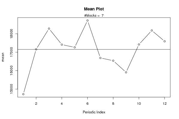
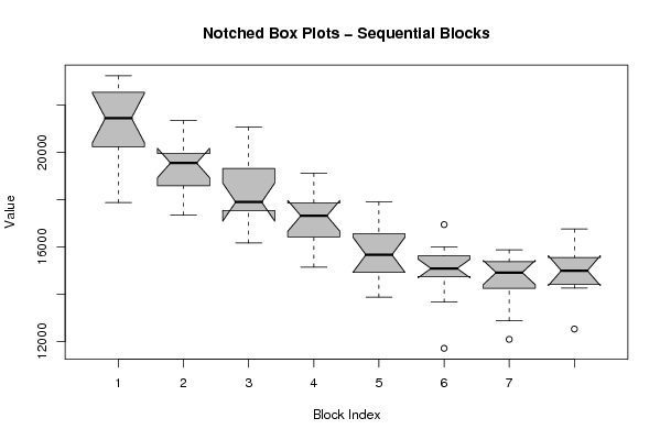
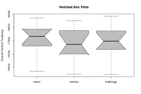
| Title produced by software | Mean Plot | ||||||||||||||||||||
| Date of computation | Wed, 10 Dec 2008 08:03:46 -0700 | ||||||||||||||||||||
| Cite this page as follows | Statistical Computations at FreeStatistics.org, Office for Research Development and Education, URL https://freestatistics.org/blog/index.php?v=date/2008/Dec/10/t122892145748pujxmhtgg5gj3.htm/, Retrieved Sun, 19 May 2024 05:13:47 +0000 | ||||||||||||||||||||
| Statistical Computations at FreeStatistics.org, Office for Research Development and Education, URL https://freestatistics.org/blog/index.php?pk=31989, Retrieved Sun, 19 May 2024 05:13:47 +0000 | |||||||||||||||||||||
| QR Codes: | |||||||||||||||||||||
|
| |||||||||||||||||||||
| Original text written by user: | |||||||||||||||||||||
| IsPrivate? | No (this computation is public) | ||||||||||||||||||||
| User-defined keywords | |||||||||||||||||||||
| Estimated Impact | 243 | ||||||||||||||||||||
Tree of Dependent Computations | |||||||||||||||||||||
| Family? (F = Feedback message, R = changed R code, M = changed R Module, P = changed Parameters, D = changed Data) | |||||||||||||||||||||
| - [Mean Plot] [Mean Plot - Uitvoer] [2008-12-10 15:03:46] [c0a347e3519123f7eef62b705326dad9] [Current] - D [Mean Plot] [Mean Plot voor ui...] [2008-12-18 23:25:01] [29747f79f5beb5b2516e1271770ecb47] | |||||||||||||||||||||
| Feedback Forum | |||||||||||||||||||||
Post a new message | |||||||||||||||||||||
Dataset | |||||||||||||||||||||
| Dataseries X: | |||||||||||||||||||||
18 562,2 23 184,8 22 925,8 21 490,2 23 243,2 21 688,7 21 423,1 21 211,2 17 877,4 20 664,3 22 160,0 19 813,6 17 735,4 19 640,2 20 844,4 19 823,1 18 594,6 21 350,6 18 574,1 18 924,2 17 343,4 19 961,2 19 932,1 19 464,6 16 165,4 17 574,9 19 795,4 19 439,5 17 170,0 21 072,4 17 751,8 17 515,5 18 040,3 19 090,1 17 746,5 19 202,1 15 141,6 16 258,1 18 586,5 17 209,4 17 838,7 19 123,5 16 583,6 15 991,2 16 704,4 17 420,4 17 872,0 17 823,2 13 866,5 15 912,8 17 870,5 15 420,3 16 379,4 17 903,9 15 305,8 14 583,3 14 861,0 14 968,9 16 726,5 16 283,6 11 703,7 15 101,8 15 469,7 14 956,9 15 370,6 15 998,1 14 725,1 14 768,9 13 659,6 15 070,3 16 943,0 15 761,3 12 083,0 15 023,6 15 106,5 15 498,6 15 258,9 15 859,4 14 205,3 14 291,1 12 875,1 14 755,3 15 873,2 14 803,0 12 520,2 14 568,3 15 644,8 15 454,9 14 254,0 16 754,8 14 944,2 15 044,5 | |||||||||||||||||||||
Tables (Output of Computation) | |||||||||||||||||||||
| |||||||||||||||||||||
Figures (Output of Computation) | |||||||||||||||||||||
Input Parameters & R Code | |||||||||||||||||||||
| Parameters (Session): | |||||||||||||||||||||
| par1 = 12 ; | |||||||||||||||||||||
| Parameters (R input): | |||||||||||||||||||||
| par1 = 12 ; | |||||||||||||||||||||
| R code (references can be found in the software module): | |||||||||||||||||||||
par1 <- as.numeric(par1) | |||||||||||||||||||||