Free Statistics
of Irreproducible Research!
Description of Statistical Computation | |||||||||||||||||||||
|---|---|---|---|---|---|---|---|---|---|---|---|---|---|---|---|---|---|---|---|---|---|
| Author's title | |||||||||||||||||||||
| Author | *The author of this computation has been verified* | ||||||||||||||||||||
| R Software Module | rwasp_meanplot.wasp | ||||||||||||||||||||
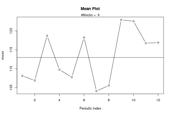
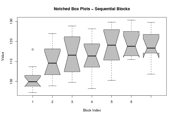
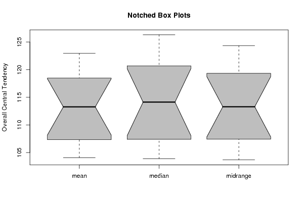
| Title produced by software | Mean Plot | ||||||||||||||||||||
| Date of computation | Wed, 10 Dec 2008 05:25:17 -0700 | ||||||||||||||||||||
| Cite this page as follows | Statistical Computations at FreeStatistics.org, Office for Research Development and Education, URL https://freestatistics.org/blog/index.php?v=date/2008/Dec/10/t1228911949cvkfgcsl8str2kw.htm/, Retrieved Sun, 19 May 2024 07:55:30 +0000 | ||||||||||||||||||||
| Statistical Computations at FreeStatistics.org, Office for Research Development and Education, URL https://freestatistics.org/blog/index.php?pk=31920, Retrieved Sun, 19 May 2024 07:55:30 +0000 | |||||||||||||||||||||
| QR Codes: | |||||||||||||||||||||
|
| |||||||||||||||||||||
| Original text written by user: | |||||||||||||||||||||
| IsPrivate? | No (this computation is public) | ||||||||||||||||||||
| User-defined keywords | |||||||||||||||||||||
| Estimated Impact | 167 | ||||||||||||||||||||
Tree of Dependent Computations | |||||||||||||||||||||
| Family? (F = Feedback message, R = changed R code, M = changed R Module, P = changed Parameters, D = changed Data) | |||||||||||||||||||||
| - [Mean Plot] [Mean Plot: Totale...] [2008-12-10 12:25:17] [b5110a3ab194da7214bdf478e0a05dbd] [Current] | |||||||||||||||||||||
| Feedback Forum | |||||||||||||||||||||
Post a new message | |||||||||||||||||||||
Dataset | |||||||||||||||||||||
| Dataseries X: | |||||||||||||||||||||
98,5 97,0 103,3 99,6 100,1 102,9 95,9 94,5 107,4 116,0 102,8 99,8 109,6 103,0 111,6 106,3 97,9 108,8 103,9 101,2 122,9 123,9 111,7 120,9 99,6 103,3 119,4 106,5 101,9 124,6 106,5 107,8 127,4 120,1 118,5 127,7 107,7 104,5 118,8 110,3 109,6 119,1 96,5 106,7 126,3 116,2 118,8 115,2 110,0 111,4 129,6 108,1 117,8 122,9 100,6 111,8 127,0 128,6 124,8 118,5 114,7 112,6 128,7 111,0 115,8 126,0 111,1 113,2 120,1 130,6 124,0 119,4 116,7 116,5 119,6 126,5 111,3 123,5 114,2 103,7 129,5 | |||||||||||||||||||||
Tables (Output of Computation) | |||||||||||||||||||||
| |||||||||||||||||||||
Figures (Output of Computation) | |||||||||||||||||||||
Input Parameters & R Code | |||||||||||||||||||||
| Parameters (Session): | |||||||||||||||||||||
| par1 = 12 ; | |||||||||||||||||||||
| Parameters (R input): | |||||||||||||||||||||
| par1 = 12 ; | |||||||||||||||||||||
| R code (references can be found in the software module): | |||||||||||||||||||||
par1 <- as.numeric(par1) | |||||||||||||||||||||