Repository of Reproducible Computations

Free Statistics

of Irreproducible Research!

Author's title

Author

*Unverified author*

R Software Module

rwasp_autocorrelation.wasp

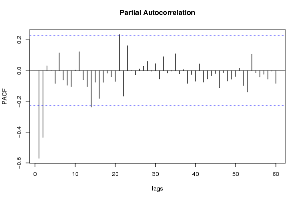
Title produced by software

(Partial) Autocorrelation Function

Date of computation

Tue, 09 Dec 2008 11:06:59 -0700

Cite this page as follows

Statistical Computations at FreeStatistics.org, Office for Research Development and Education, URL https://freestatistics.org/blog/index.php?v=date/2008/Dec/09/t1228846043u1qlalklo3lhwlr.htm/, Retrieved Sun, 19 May 2024 10:23:08 +0000

Statistical Computations at FreeStatistics.org, Office for Research Development and Education, URL https://freestatistics.org/blog/index.php?pk=31652, Retrieved Sun, 19 May 2024 10:23:08 +0000

QR Codes:

Paste this QR Code to cite your computation.

Original text written by user:

IsPrivate?

No (this computation is public)

User-defined keywords

Estimated Impact

173

Family? (F = Feedback message, R = changed R code, M = changed R Module, P = changed Parameters, D = changed Data)

-     [Univariate Data Series] [data set] [2008-12-01 19:54:57] [b98453cac15ba1066b407e146608df68]
- RMP   [(Partial) Autocorrelation Function] [Gilliam Schoorel] [2008-12-07 20:50:54] [a9b974cca921a7a5a84c6ce01f3dc8c2]
F R  D      [(Partial) Autocorrelation Function] [] [2008-12-09 18:06:59] [d41d8cd98f00b204e9800998ecf8427e] [Current]

Feedback Forum

2008-12-13 22:51:19 [Li Tang Hu] [reply] 
je hebt een betrouwbaarheidsinterval van 95% waardoor dus 5% er eventueel mag uitschieten...in dit geval maken die 4 uitschieters dus niet zoveel uit

Post a new message

Dataseries X:

Download CSV

Histogram

Boxplots

Summary of computational transaction
Raw Input	view raw input (R code)
Raw Output	view raw output of R engine
Computing time	1 seconds
R Server	'George Udny Yule' @ 72.249.76.132

\begin{tabular}{lllllllll}
\hline
Summary of computational transaction \tabularnewline
Raw Input & view raw input (R code)  \tabularnewline
Raw Output & view raw output of R engine  \tabularnewline
Computing time & 1 seconds \tabularnewline
R Server & 'George Udny Yule' @ 72.249.76.132 \tabularnewline
\hline
\end{tabular}
%Source: https://freestatistics.org/blog/index.php?pk=31652&T=0

[TABLE]
[ROW][C]Summary of computational transaction[/C][/ROW]
[ROW][C]Raw Input[/C][C]view raw input (R code) [/C][/ROW]
[ROW][C]Raw Output[/C][C]view raw output of R engine [/C][/ROW]
[ROW][C]Computing time[/C][C]1 seconds[/C][/ROW]
[ROW][C]R Server[/C][C]'George Udny Yule' @ 72.249.76.132[/C][/ROW]
[/TABLE]
Source: https://freestatistics.org/blog/index.php?pk=31652&T=0

Globally Unique Identifier (entire table): ba.freestatistics.org/blog/index.php?pk=31652&T=0

As an alternative you can also use a QR Code:

The GUIDs for individual cells are displayed in the table below:

Summary of computational transaction
Raw Input	view raw input (R code)
Raw Output	view raw output of R engine
Computing time	1 seconds
R Server	'George Udny Yule' @ 72.249.76.132

Autocorrelation Function
Time lag k	ACF(k)	T-STAT	P-value
1	-0.569951	-4.9359	2e-06
2	0.031238	0.2705	0.39375
3	0.239259	2.072	0.02085
4	-0.223218	-1.9331	0.028498
5	0.036848	0.3191	0.375263
6	0.168424	1.4586	0.074426
7	-0.250651	-2.1707	0.016559
8	0.116796	1.0115	0.157519
9	0.008917	0.0772	0.469326
10	-0.051162	-0.4431	0.329494
11	0.097393	0.8434	0.20083
12	-0.124986	-1.0824	0.141269
13	0.026048	0.2256	0.41107
14	-0.033114	-0.2868	0.387537
15	0.051971	0.4501	0.326974
16	-0.107046	-0.927	0.178438
17	0.091685	0.794	0.214847
18	-0.041812	-0.3621	0.359147
19	-0.012018	-0.1041	0.458692
20	0.03736	0.3235	0.373591
21	0.145459	1.2597	0.10584
22	-0.342854	-2.9692	0.002004
23	0.398668	3.4526	0.000458
24	-0.227888	-1.9736	0.026058
25	-0.031564	-0.2734	0.392666
26	0.216161	1.872	0.032552
27	-0.169477	-1.4677	0.073182
28	0.01983	0.1717	0.432055
29	0.127602	1.1051	0.136332
30	-0.129127	-1.1183	0.13351
31	0.020409	0.1767	0.430092
32	0.123263	1.0675	0.144588
33	-0.225217	-1.9504	0.02743
34	0.169016	1.4637	0.073724
35	-0.043561	-0.3773	0.353525
36	-0.0789	-0.6833	0.248264
37	0.072427	0.6272	0.266204
38	-0.019883	-0.1722	0.431874
39	-0.078936	-0.6836	0.248165
40	0.10469	0.9066	0.183751
41	-0.040554	-0.3512	0.36321
42	-0.065207	-0.5647	0.286978
43	0.055092	0.4771	0.317337
44	0.045373	0.3929	0.347739
45	-0.135557	-1.174	0.122063
46	0.124027	1.0741	0.143109
47	-0.012426	-0.1076	0.457296
48	-0.112735	-0.9763	0.166023
49	0.169833	1.4708	0.072765
50	-0.087107	-0.7544	0.226494
51	0.01085	0.094	0.462693
52	0.01404	0.1216	0.451774
53	-0.022043	-0.1909	0.424562
54	0.058257	0.5045	0.307688
55	0.004211	0.0365	0.485504
56	-0.108686	-0.9413	0.174799
57	0.119297	1.0331	0.152429
58	-0.050887	-0.4407	0.330352
59	-0.041377	-0.3583	0.360551
60	0.081712	0.7076	0.24068

\begin{tabular}{lllllllll}
\hline
Autocorrelation Function \tabularnewline
Time lag k & ACF(k) & T-STAT & P-value \tabularnewline
1 & -0.569951 & -4.9359 & 2e-06 \tabularnewline
2 & 0.031238 & 0.2705 & 0.39375 \tabularnewline
3 & 0.239259 & 2.072 & 0.02085 \tabularnewline
4 & -0.223218 & -1.9331 & 0.028498 \tabularnewline
5 & 0.036848 & 0.3191 & 0.375263 \tabularnewline
6 & 0.168424 & 1.4586 & 0.074426 \tabularnewline
7 & -0.250651 & -2.1707 & 0.016559 \tabularnewline
8 & 0.116796 & 1.0115 & 0.157519 \tabularnewline
9 & 0.008917 & 0.0772 & 0.469326 \tabularnewline
10 & -0.051162 & -0.4431 & 0.329494 \tabularnewline
11 & 0.097393 & 0.8434 & 0.20083 \tabularnewline
12 & -0.124986 & -1.0824 & 0.141269 \tabularnewline
13 & 0.026048 & 0.2256 & 0.41107 \tabularnewline
14 & -0.033114 & -0.2868 & 0.387537 \tabularnewline
15 & 0.051971 & 0.4501 & 0.326974 \tabularnewline
16 & -0.107046 & -0.927 & 0.178438 \tabularnewline
17 & 0.091685 & 0.794 & 0.214847 \tabularnewline
18 & -0.041812 & -0.3621 & 0.359147 \tabularnewline
19 & -0.012018 & -0.1041 & 0.458692 \tabularnewline
20 & 0.03736 & 0.3235 & 0.373591 \tabularnewline
21 & 0.145459 & 1.2597 & 0.10584 \tabularnewline
22 & -0.342854 & -2.9692 & 0.002004 \tabularnewline
23 & 0.398668 & 3.4526 & 0.000458 \tabularnewline
24 & -0.227888 & -1.9736 & 0.026058 \tabularnewline
25 & -0.031564 & -0.2734 & 0.392666 \tabularnewline
26 & 0.216161 & 1.872 & 0.032552 \tabularnewline
27 & -0.169477 & -1.4677 & 0.073182 \tabularnewline
28 & 0.01983 & 0.1717 & 0.432055 \tabularnewline
29 & 0.127602 & 1.1051 & 0.136332 \tabularnewline
30 & -0.129127 & -1.1183 & 0.13351 \tabularnewline
31 & 0.020409 & 0.1767 & 0.430092 \tabularnewline
32 & 0.123263 & 1.0675 & 0.144588 \tabularnewline
33 & -0.225217 & -1.9504 & 0.02743 \tabularnewline
34 & 0.169016 & 1.4637 & 0.073724 \tabularnewline
35 & -0.043561 & -0.3773 & 0.353525 \tabularnewline
36 & -0.0789 & -0.6833 & 0.248264 \tabularnewline
37 & 0.072427 & 0.6272 & 0.266204 \tabularnewline
38 & -0.019883 & -0.1722 & 0.431874 \tabularnewline
39 & -0.078936 & -0.6836 & 0.248165 \tabularnewline
40 & 0.10469 & 0.9066 & 0.183751 \tabularnewline
41 & -0.040554 & -0.3512 & 0.36321 \tabularnewline
42 & -0.065207 & -0.5647 & 0.286978 \tabularnewline
43 & 0.055092 & 0.4771 & 0.317337 \tabularnewline
44 & 0.045373 & 0.3929 & 0.347739 \tabularnewline
45 & -0.135557 & -1.174 & 0.122063 \tabularnewline
46 & 0.124027 & 1.0741 & 0.143109 \tabularnewline
47 & -0.012426 & -0.1076 & 0.457296 \tabularnewline
48 & -0.112735 & -0.9763 & 0.166023 \tabularnewline
49 & 0.169833 & 1.4708 & 0.072765 \tabularnewline
50 & -0.087107 & -0.7544 & 0.226494 \tabularnewline
51 & 0.01085 & 0.094 & 0.462693 \tabularnewline
52 & 0.01404 & 0.1216 & 0.451774 \tabularnewline
53 & -0.022043 & -0.1909 & 0.424562 \tabularnewline
54 & 0.058257 & 0.5045 & 0.307688 \tabularnewline
55 & 0.004211 & 0.0365 & 0.485504 \tabularnewline
56 & -0.108686 & -0.9413 & 0.174799 \tabularnewline
57 & 0.119297 & 1.0331 & 0.152429 \tabularnewline
58 & -0.050887 & -0.4407 & 0.330352 \tabularnewline
59 & -0.041377 & -0.3583 & 0.360551 \tabularnewline
60 & 0.081712 & 0.7076 & 0.24068 \tabularnewline
\hline
\end{tabular}
%Source: https://freestatistics.org/blog/index.php?pk=31652&T=1

[TABLE]
[ROW][C]Autocorrelation Function[/C][/ROW]
[ROW][C]Time lag k[/C][C]ACF(k)[/C][C]T-STAT[/C][C]P-value[/C][/ROW]
[ROW][C]1[/C][C]-0.569951[/C][C]-4.9359[/C][C]2e-06[/C][/ROW]
[ROW][C]2[/C][C]0.031238[/C][C]0.2705[/C][C]0.39375[/C][/ROW]
[ROW][C]3[/C][C]0.239259[/C][C]2.072[/C][C]0.02085[/C][/ROW]
[ROW][C]4[/C][C]-0.223218[/C][C]-1.9331[/C][C]0.028498[/C][/ROW]
[ROW][C]5[/C][C]0.036848[/C][C]0.3191[/C][C]0.375263[/C][/ROW]
[ROW][C]6[/C][C]0.168424[/C][C]1.4586[/C][C]0.074426[/C][/ROW]
[ROW][C]7[/C][C]-0.250651[/C][C]-2.1707[/C][C]0.016559[/C][/ROW]
[ROW][C]8[/C][C]0.116796[/C][C]1.0115[/C][C]0.157519[/C][/ROW]
[ROW][C]9[/C][C]0.008917[/C][C]0.0772[/C][C]0.469326[/C][/ROW]
[ROW][C]10[/C][C]-0.051162[/C][C]-0.4431[/C][C]0.329494[/C][/ROW]
[ROW][C]11[/C][C]0.097393[/C][C]0.8434[/C][C]0.20083[/C][/ROW]
[ROW][C]12[/C][C]-0.124986[/C][C]-1.0824[/C][C]0.141269[/C][/ROW]
[ROW][C]13[/C][C]0.026048[/C][C]0.2256[/C][C]0.41107[/C][/ROW]
[ROW][C]14[/C][C]-0.033114[/C][C]-0.2868[/C][C]0.387537[/C][/ROW]
[ROW][C]15[/C][C]0.051971[/C][C]0.4501[/C][C]0.326974[/C][/ROW]
[ROW][C]16[/C][C]-0.107046[/C][C]-0.927[/C][C]0.178438[/C][/ROW]
[ROW][C]17[/C][C]0.091685[/C][C]0.794[/C][C]0.214847[/C][/ROW]
[ROW][C]18[/C][C]-0.041812[/C][C]-0.3621[/C][C]0.359147[/C][/ROW]
[ROW][C]19[/C][C]-0.012018[/C][C]-0.1041[/C][C]0.458692[/C][/ROW]
[ROW][C]20[/C][C]0.03736[/C][C]0.3235[/C][C]0.373591[/C][/ROW]
[ROW][C]21[/C][C]0.145459[/C][C]1.2597[/C][C]0.10584[/C][/ROW]
[ROW][C]22[/C][C]-0.342854[/C][C]-2.9692[/C][C]0.002004[/C][/ROW]
[ROW][C]23[/C][C]0.398668[/C][C]3.4526[/C][C]0.000458[/C][/ROW]
[ROW][C]24[/C][C]-0.227888[/C][C]-1.9736[/C][C]0.026058[/C][/ROW]
[ROW][C]25[/C][C]-0.031564[/C][C]-0.2734[/C][C]0.392666[/C][/ROW]
[ROW][C]26[/C][C]0.216161[/C][C]1.872[/C][C]0.032552[/C][/ROW]
[ROW][C]27[/C][C]-0.169477[/C][C]-1.4677[/C][C]0.073182[/C][/ROW]
[ROW][C]28[/C][C]0.01983[/C][C]0.1717[/C][C]0.432055[/C][/ROW]
[ROW][C]29[/C][C]0.127602[/C][C]1.1051[/C][C]0.136332[/C][/ROW]
[ROW][C]30[/C][C]-0.129127[/C][C]-1.1183[/C][C]0.13351[/C][/ROW]
[ROW][C]31[/C][C]0.020409[/C][C]0.1767[/C][C]0.430092[/C][/ROW]
[ROW][C]32[/C][C]0.123263[/C][C]1.0675[/C][C]0.144588[/C][/ROW]
[ROW][C]33[/C][C]-0.225217[/C][C]-1.9504[/C][C]0.02743[/C][/ROW]
[ROW][C]34[/C][C]0.169016[/C][C]1.4637[/C][C]0.073724[/C][/ROW]
[ROW][C]35[/C][C]-0.043561[/C][C]-0.3773[/C][C]0.353525[/C][/ROW]
[ROW][C]36[/C][C]-0.0789[/C][C]-0.6833[/C][C]0.248264[/C][/ROW]
[ROW][C]37[/C][C]0.072427[/C][C]0.6272[/C][C]0.266204[/C][/ROW]
[ROW][C]38[/C][C]-0.019883[/C][C]-0.1722[/C][C]0.431874[/C][/ROW]
[ROW][C]39[/C][C]-0.078936[/C][C]-0.6836[/C][C]0.248165[/C][/ROW]
[ROW][C]40[/C][C]0.10469[/C][C]0.9066[/C][C]0.183751[/C][/ROW]
[ROW][C]41[/C][C]-0.040554[/C][C]-0.3512[/C][C]0.36321[/C][/ROW]
[ROW][C]42[/C][C]-0.065207[/C][C]-0.5647[/C][C]0.286978[/C][/ROW]
[ROW][C]43[/C][C]0.055092[/C][C]0.4771[/C][C]0.317337[/C][/ROW]
[ROW][C]44[/C][C]0.045373[/C][C]0.3929[/C][C]0.347739[/C][/ROW]
[ROW][C]45[/C][C]-0.135557[/C][C]-1.174[/C][C]0.122063[/C][/ROW]
[ROW][C]46[/C][C]0.124027[/C][C]1.0741[/C][C]0.143109[/C][/ROW]
[ROW][C]47[/C][C]-0.012426[/C][C]-0.1076[/C][C]0.457296[/C][/ROW]
[ROW][C]48[/C][C]-0.112735[/C][C]-0.9763[/C][C]0.166023[/C][/ROW]
[ROW][C]49[/C][C]0.169833[/C][C]1.4708[/C][C]0.072765[/C][/ROW]
[ROW][C]50[/C][C]-0.087107[/C][C]-0.7544[/C][C]0.226494[/C][/ROW]
[ROW][C]51[/C][C]0.01085[/C][C]0.094[/C][C]0.462693[/C][/ROW]
[ROW][C]52[/C][C]0.01404[/C][C]0.1216[/C][C]0.451774[/C][/ROW]
[ROW][C]53[/C][C]-0.022043[/C][C]-0.1909[/C][C]0.424562[/C][/ROW]
[ROW][C]54[/C][C]0.058257[/C][C]0.5045[/C][C]0.307688[/C][/ROW]
[ROW][C]55[/C][C]0.004211[/C][C]0.0365[/C][C]0.485504[/C][/ROW]
[ROW][C]56[/C][C]-0.108686[/C][C]-0.9413[/C][C]0.174799[/C][/ROW]
[ROW][C]57[/C][C]0.119297[/C][C]1.0331[/C][C]0.152429[/C][/ROW]
[ROW][C]58[/C][C]-0.050887[/C][C]-0.4407[/C][C]0.330352[/C][/ROW]
[ROW][C]59[/C][C]-0.041377[/C][C]-0.3583[/C][C]0.360551[/C][/ROW]
[ROW][C]60[/C][C]0.081712[/C][C]0.7076[/C][C]0.24068[/C][/ROW]
[/TABLE]
Source: https://freestatistics.org/blog/index.php?pk=31652&T=1

Globally Unique Identifier (entire table): ba.freestatistics.org/blog/index.php?pk=31652&T=1

As an alternative you can also use a QR Code:

The GUIDs for individual cells are displayed in the table below:

Autocorrelation Function
Time lag k	ACF(k)	T-STAT	P-value
1	-0.569951	-4.9359	2e-06
2	0.031238	0.2705	0.39375
3	0.239259	2.072	0.02085
4	-0.223218	-1.9331	0.028498
5	0.036848	0.3191	0.375263
6	0.168424	1.4586	0.074426
7	-0.250651	-2.1707	0.016559
8	0.116796	1.0115	0.157519
9	0.008917	0.0772	0.469326
10	-0.051162	-0.4431	0.329494
11	0.097393	0.8434	0.20083
12	-0.124986	-1.0824	0.141269
13	0.026048	0.2256	0.41107
14	-0.033114	-0.2868	0.387537
15	0.051971	0.4501	0.326974
16	-0.107046	-0.927	0.178438
17	0.091685	0.794	0.214847
18	-0.041812	-0.3621	0.359147
19	-0.012018	-0.1041	0.458692
20	0.03736	0.3235	0.373591
21	0.145459	1.2597	0.10584
22	-0.342854	-2.9692	0.002004
23	0.398668	3.4526	0.000458
24	-0.227888	-1.9736	0.026058
25	-0.031564	-0.2734	0.392666
26	0.216161	1.872	0.032552
27	-0.169477	-1.4677	0.073182
28	0.01983	0.1717	0.432055
29	0.127602	1.1051	0.136332
30	-0.129127	-1.1183	0.13351
31	0.020409	0.1767	0.430092
32	0.123263	1.0675	0.144588
33	-0.225217	-1.9504	0.02743
34	0.169016	1.4637	0.073724
35	-0.043561	-0.3773	0.353525
36	-0.0789	-0.6833	0.248264
37	0.072427	0.6272	0.266204
38	-0.019883	-0.1722	0.431874
39	-0.078936	-0.6836	0.248165
40	0.10469	0.9066	0.183751
41	-0.040554	-0.3512	0.36321
42	-0.065207	-0.5647	0.286978
43	0.055092	0.4771	0.317337
44	0.045373	0.3929	0.347739
45	-0.135557	-1.174	0.122063
46	0.124027	1.0741	0.143109
47	-0.012426	-0.1076	0.457296
48	-0.112735	-0.9763	0.166023
49	0.169833	1.4708	0.072765
50	-0.087107	-0.7544	0.226494
51	0.01085	0.094	0.462693
52	0.01404	0.1216	0.451774
53	-0.022043	-0.1909	0.424562
54	0.058257	0.5045	0.307688
55	0.004211	0.0365	0.485504
56	-0.108686	-0.9413	0.174799
57	0.119297	1.0331	0.152429
58	-0.050887	-0.4407	0.330352
59	-0.041377	-0.3583	0.360551
60	0.081712	0.7076	0.24068

Partial Autocorrelation Function
Time lag k	PACF(k)	T-STAT	P-value
1	-0.569951	-4.9359	2e-06
2	-0.434871	-3.7661	0.000164
3	0.030961	0.2681	0.394668
4	-0.000607	-0.0053	0.497911
5	-0.083993	-0.7274	0.234623
6	0.114828	0.9944	0.161602
7	-0.060747	-0.5261	0.300191
8	-0.095547	-0.8275	0.205301
9	-0.10493	-0.9087	0.183204
10	0.003886	0.0337	0.48662
11	0.122733	1.0629	0.145619
12	-0.060386	-0.523	0.301273
13	-0.104751	-0.9072	0.183611
14	-0.236817	-2.0509	0.021885
15	-0.075403	-0.653	0.257873
16	-0.181472	-1.5716	0.060127
17	-0.076268	-0.6605	0.255478
18	-0.016682	-0.1445	0.442757
19	-0.040982	-0.3549	0.361826
20	-0.07098	-0.6147	0.270305
21	0.234681	2.0324	0.022827
22	-0.165531	-1.4335	0.07793
23	0.162237	1.405	0.082073
24	0.000428	0.0037	0.498527
25	-0.028159	-0.2439	0.403999
26	0.01047	0.0907	0.463998
27	0.029231	0.2531	0.400424
28	0.060419	0.5232	0.301174
29	-0.003323	-0.0288	0.488559
30	0.04552	0.3942	0.347271
31	-0.054372	-0.4709	0.319548
32	0.090635	0.7849	0.217485
33	-0.015497	-0.1342	0.446799
34	-0.003003	-0.026	0.489661
35	0.109525	0.9485	0.172956
36	-0.020945	-0.1814	0.428276
37	0.007067	0.0612	0.475679
38	-0.083583	-0.7238	0.235705
39	-0.025993	-0.2251	0.411253
40	-0.06926	-0.5998	0.275222
41	0.043504	0.3768	0.353709
42	-0.07449	-0.6451	0.260416
43	-0.054237	-0.4697	0.319965
44	-0.033706	-0.2919	0.385584
45	-0.019556	-0.1694	0.432986
46	-0.112365	-0.9731	0.166814
47	-0.013882	-0.1202	0.452316
48	-0.067665	-0.586	0.27982
49	-0.056033	-0.4853	0.314454
50	-0.038859	-0.3365	0.368706
51	0.015892	0.1376	0.44545
52	-0.097775	-0.8468	0.199912
53	-0.138957	-1.2034	0.116303
54	0.10674	0.9244	0.179124
55	-0.014447	-0.1251	0.450384
56	-0.041299	-0.3577	0.360802
57	-0.023959	-0.2075	0.418094
58	-0.055121	-0.4774	0.317246
59	-0.003782	-0.0328	0.486978
60	-0.083607	-0.7241	0.23564

\begin{tabular}{lllllllll}
\hline
Partial Autocorrelation Function \tabularnewline
Time lag k & PACF(k) & T-STAT & P-value \tabularnewline
1 & -0.569951 & -4.9359 & 2e-06 \tabularnewline
2 & -0.434871 & -3.7661 & 0.000164 \tabularnewline
3 & 0.030961 & 0.2681 & 0.394668 \tabularnewline
4 & -0.000607 & -0.0053 & 0.497911 \tabularnewline
5 & -0.083993 & -0.7274 & 0.234623 \tabularnewline
6 & 0.114828 & 0.9944 & 0.161602 \tabularnewline
7 & -0.060747 & -0.5261 & 0.300191 \tabularnewline
8 & -0.095547 & -0.8275 & 0.205301 \tabularnewline
9 & -0.10493 & -0.9087 & 0.183204 \tabularnewline
10 & 0.003886 & 0.0337 & 0.48662 \tabularnewline
11 & 0.122733 & 1.0629 & 0.145619 \tabularnewline
12 & -0.060386 & -0.523 & 0.301273 \tabularnewline
13 & -0.104751 & -0.9072 & 0.183611 \tabularnewline
14 & -0.236817 & -2.0509 & 0.021885 \tabularnewline
15 & -0.075403 & -0.653 & 0.257873 \tabularnewline
16 & -0.181472 & -1.5716 & 0.060127 \tabularnewline
17 & -0.076268 & -0.6605 & 0.255478 \tabularnewline
18 & -0.016682 & -0.1445 & 0.442757 \tabularnewline
19 & -0.040982 & -0.3549 & 0.361826 \tabularnewline
20 & -0.07098 & -0.6147 & 0.270305 \tabularnewline
21 & 0.234681 & 2.0324 & 0.022827 \tabularnewline
22 & -0.165531 & -1.4335 & 0.07793 \tabularnewline
23 & 0.162237 & 1.405 & 0.082073 \tabularnewline
24 & 0.000428 & 0.0037 & 0.498527 \tabularnewline
25 & -0.028159 & -0.2439 & 0.403999 \tabularnewline
26 & 0.01047 & 0.0907 & 0.463998 \tabularnewline
27 & 0.029231 & 0.2531 & 0.400424 \tabularnewline
28 & 0.060419 & 0.5232 & 0.301174 \tabularnewline
29 & -0.003323 & -0.0288 & 0.488559 \tabularnewline
30 & 0.04552 & 0.3942 & 0.347271 \tabularnewline
31 & -0.054372 & -0.4709 & 0.319548 \tabularnewline
32 & 0.090635 & 0.7849 & 0.217485 \tabularnewline
33 & -0.015497 & -0.1342 & 0.446799 \tabularnewline
34 & -0.003003 & -0.026 & 0.489661 \tabularnewline
35 & 0.109525 & 0.9485 & 0.172956 \tabularnewline
36 & -0.020945 & -0.1814 & 0.428276 \tabularnewline
37 & 0.007067 & 0.0612 & 0.475679 \tabularnewline
38 & -0.083583 & -0.7238 & 0.235705 \tabularnewline
39 & -0.025993 & -0.2251 & 0.411253 \tabularnewline
40 & -0.06926 & -0.5998 & 0.275222 \tabularnewline
41 & 0.043504 & 0.3768 & 0.353709 \tabularnewline
42 & -0.07449 & -0.6451 & 0.260416 \tabularnewline
43 & -0.054237 & -0.4697 & 0.319965 \tabularnewline
44 & -0.033706 & -0.2919 & 0.385584 \tabularnewline
45 & -0.019556 & -0.1694 & 0.432986 \tabularnewline
46 & -0.112365 & -0.9731 & 0.166814 \tabularnewline
47 & -0.013882 & -0.1202 & 0.452316 \tabularnewline
48 & -0.067665 & -0.586 & 0.27982 \tabularnewline
49 & -0.056033 & -0.4853 & 0.314454 \tabularnewline
50 & -0.038859 & -0.3365 & 0.368706 \tabularnewline
51 & 0.015892 & 0.1376 & 0.44545 \tabularnewline
52 & -0.097775 & -0.8468 & 0.199912 \tabularnewline
53 & -0.138957 & -1.2034 & 0.116303 \tabularnewline
54 & 0.10674 & 0.9244 & 0.179124 \tabularnewline
55 & -0.014447 & -0.1251 & 0.450384 \tabularnewline
56 & -0.041299 & -0.3577 & 0.360802 \tabularnewline
57 & -0.023959 & -0.2075 & 0.418094 \tabularnewline
58 & -0.055121 & -0.4774 & 0.317246 \tabularnewline
59 & -0.003782 & -0.0328 & 0.486978 \tabularnewline
60 & -0.083607 & -0.7241 & 0.23564 \tabularnewline
\hline
\end{tabular}
%Source: https://freestatistics.org/blog/index.php?pk=31652&T=2

[TABLE]
[ROW][C]Partial Autocorrelation Function[/C][/ROW]
[ROW][C]Time lag k[/C][C]PACF(k)[/C][C]T-STAT[/C][C]P-value[/C][/ROW]
[ROW][C]1[/C][C]-0.569951[/C][C]-4.9359[/C][C]2e-06[/C][/ROW]
[ROW][C]2[/C][C]-0.434871[/C][C]-3.7661[/C][C]0.000164[/C][/ROW]
[ROW][C]3[/C][C]0.030961[/C][C]0.2681[/C][C]0.394668[/C][/ROW]
[ROW][C]4[/C][C]-0.000607[/C][C]-0.0053[/C][C]0.497911[/C][/ROW]
[ROW][C]5[/C][C]-0.083993[/C][C]-0.7274[/C][C]0.234623[/C][/ROW]
[ROW][C]6[/C][C]0.114828[/C][C]0.9944[/C][C]0.161602[/C][/ROW]
[ROW][C]7[/C][C]-0.060747[/C][C]-0.5261[/C][C]0.300191[/C][/ROW]
[ROW][C]8[/C][C]-0.095547[/C][C]-0.8275[/C][C]0.205301[/C][/ROW]
[ROW][C]9[/C][C]-0.10493[/C][C]-0.9087[/C][C]0.183204[/C][/ROW]
[ROW][C]10[/C][C]0.003886[/C][C]0.0337[/C][C]0.48662[/C][/ROW]
[ROW][C]11[/C][C]0.122733[/C][C]1.0629[/C][C]0.145619[/C][/ROW]
[ROW][C]12[/C][C]-0.060386[/C][C]-0.523[/C][C]0.301273[/C][/ROW]
[ROW][C]13[/C][C]-0.104751[/C][C]-0.9072[/C][C]0.183611[/C][/ROW]
[ROW][C]14[/C][C]-0.236817[/C][C]-2.0509[/C][C]0.021885[/C][/ROW]
[ROW][C]15[/C][C]-0.075403[/C][C]-0.653[/C][C]0.257873[/C][/ROW]
[ROW][C]16[/C][C]-0.181472[/C][C]-1.5716[/C][C]0.060127[/C][/ROW]
[ROW][C]17[/C][C]-0.076268[/C][C]-0.6605[/C][C]0.255478[/C][/ROW]
[ROW][C]18[/C][C]-0.016682[/C][C]-0.1445[/C][C]0.442757[/C][/ROW]
[ROW][C]19[/C][C]-0.040982[/C][C]-0.3549[/C][C]0.361826[/C][/ROW]
[ROW][C]20[/C][C]-0.07098[/C][C]-0.6147[/C][C]0.270305[/C][/ROW]
[ROW][C]21[/C][C]0.234681[/C][C]2.0324[/C][C]0.022827[/C][/ROW]
[ROW][C]22[/C][C]-0.165531[/C][C]-1.4335[/C][C]0.07793[/C][/ROW]
[ROW][C]23[/C][C]0.162237[/C][C]1.405[/C][C]0.082073[/C][/ROW]
[ROW][C]24[/C][C]0.000428[/C][C]0.0037[/C][C]0.498527[/C][/ROW]
[ROW][C]25[/C][C]-0.028159[/C][C]-0.2439[/C][C]0.403999[/C][/ROW]
[ROW][C]26[/C][C]0.01047[/C][C]0.0907[/C][C]0.463998[/C][/ROW]
[ROW][C]27[/C][C]0.029231[/C][C]0.2531[/C][C]0.400424[/C][/ROW]
[ROW][C]28[/C][C]0.060419[/C][C]0.5232[/C][C]0.301174[/C][/ROW]
[ROW][C]29[/C][C]-0.003323[/C][C]-0.0288[/C][C]0.488559[/C][/ROW]
[ROW][C]30[/C][C]0.04552[/C][C]0.3942[/C][C]0.347271[/C][/ROW]
[ROW][C]31[/C][C]-0.054372[/C][C]-0.4709[/C][C]0.319548[/C][/ROW]
[ROW][C]32[/C][C]0.090635[/C][C]0.7849[/C][C]0.217485[/C][/ROW]
[ROW][C]33[/C][C]-0.015497[/C][C]-0.1342[/C][C]0.446799[/C][/ROW]
[ROW][C]34[/C][C]-0.003003[/C][C]-0.026[/C][C]0.489661[/C][/ROW]
[ROW][C]35[/C][C]0.109525[/C][C]0.9485[/C][C]0.172956[/C][/ROW]
[ROW][C]36[/C][C]-0.020945[/C][C]-0.1814[/C][C]0.428276[/C][/ROW]
[ROW][C]37[/C][C]0.007067[/C][C]0.0612[/C][C]0.475679[/C][/ROW]
[ROW][C]38[/C][C]-0.083583[/C][C]-0.7238[/C][C]0.235705[/C][/ROW]
[ROW][C]39[/C][C]-0.025993[/C][C]-0.2251[/C][C]0.411253[/C][/ROW]
[ROW][C]40[/C][C]-0.06926[/C][C]-0.5998[/C][C]0.275222[/C][/ROW]
[ROW][C]41[/C][C]0.043504[/C][C]0.3768[/C][C]0.353709[/C][/ROW]
[ROW][C]42[/C][C]-0.07449[/C][C]-0.6451[/C][C]0.260416[/C][/ROW]
[ROW][C]43[/C][C]-0.054237[/C][C]-0.4697[/C][C]0.319965[/C][/ROW]
[ROW][C]44[/C][C]-0.033706[/C][C]-0.2919[/C][C]0.385584[/C][/ROW]
[ROW][C]45[/C][C]-0.019556[/C][C]-0.1694[/C][C]0.432986[/C][/ROW]
[ROW][C]46[/C][C]-0.112365[/C][C]-0.9731[/C][C]0.166814[/C][/ROW]
[ROW][C]47[/C][C]-0.013882[/C][C]-0.1202[/C][C]0.452316[/C][/ROW]
[ROW][C]48[/C][C]-0.067665[/C][C]-0.586[/C][C]0.27982[/C][/ROW]
[ROW][C]49[/C][C]-0.056033[/C][C]-0.4853[/C][C]0.314454[/C][/ROW]
[ROW][C]50[/C][C]-0.038859[/C][C]-0.3365[/C][C]0.368706[/C][/ROW]
[ROW][C]51[/C][C]0.015892[/C][C]0.1376[/C][C]0.44545[/C][/ROW]
[ROW][C]52[/C][C]-0.097775[/C][C]-0.8468[/C][C]0.199912[/C][/ROW]
[ROW][C]53[/C][C]-0.138957[/C][C]-1.2034[/C][C]0.116303[/C][/ROW]
[ROW][C]54[/C][C]0.10674[/C][C]0.9244[/C][C]0.179124[/C][/ROW]
[ROW][C]55[/C][C]-0.014447[/C][C]-0.1251[/C][C]0.450384[/C][/ROW]
[ROW][C]56[/C][C]-0.041299[/C][C]-0.3577[/C][C]0.360802[/C][/ROW]
[ROW][C]57[/C][C]-0.023959[/C][C]-0.2075[/C][C]0.418094[/C][/ROW]
[ROW][C]58[/C][C]-0.055121[/C][C]-0.4774[/C][C]0.317246[/C][/ROW]
[ROW][C]59[/C][C]-0.003782[/C][C]-0.0328[/C][C]0.486978[/C][/ROW]
[ROW][C]60[/C][C]-0.083607[/C][C]-0.7241[/C][C]0.23564[/C][/ROW]
[/TABLE]
Source: https://freestatistics.org/blog/index.php?pk=31652&T=2

Globally Unique Identifier (entire table): ba.freestatistics.org/blog/index.php?pk=31652&T=2

As an alternative you can also use a QR Code:

The GUIDs for individual cells are displayed in the table below:

Partial Autocorrelation Function
Time lag k	PACF(k)	T-STAT	P-value
1	-0.569951	-4.9359	2e-06
2	-0.434871	-3.7661	0.000164
3	0.030961	0.2681	0.394668
4	-0.000607	-0.0053	0.497911
5	-0.083993	-0.7274	0.234623
6	0.114828	0.9944	0.161602
7	-0.060747	-0.5261	0.300191
8	-0.095547	-0.8275	0.205301
9	-0.10493	-0.9087	0.183204
10	0.003886	0.0337	0.48662
11	0.122733	1.0629	0.145619
12	-0.060386	-0.523	0.301273
13	-0.104751	-0.9072	0.183611
14	-0.236817	-2.0509	0.021885
15	-0.075403	-0.653	0.257873
16	-0.181472	-1.5716	0.060127
17	-0.076268	-0.6605	0.255478
18	-0.016682	-0.1445	0.442757
19	-0.040982	-0.3549	0.361826
20	-0.07098	-0.6147	0.270305
21	0.234681	2.0324	0.022827
22	-0.165531	-1.4335	0.07793
23	0.162237	1.405	0.082073
24	0.000428	0.0037	0.498527
25	-0.028159	-0.2439	0.403999
26	0.01047	0.0907	0.463998
27	0.029231	0.2531	0.400424
28	0.060419	0.5232	0.301174
29	-0.003323	-0.0288	0.488559
30	0.04552	0.3942	0.347271
31	-0.054372	-0.4709	0.319548
32	0.090635	0.7849	0.217485
33	-0.015497	-0.1342	0.446799
34	-0.003003	-0.026	0.489661
35	0.109525	0.9485	0.172956
36	-0.020945	-0.1814	0.428276
37	0.007067	0.0612	0.475679
38	-0.083583	-0.7238	0.235705
39	-0.025993	-0.2251	0.411253
40	-0.06926	-0.5998	0.275222
41	0.043504	0.3768	0.353709
42	-0.07449	-0.6451	0.260416
43	-0.054237	-0.4697	0.319965
44	-0.033706	-0.2919	0.385584
45	-0.019556	-0.1694	0.432986
46	-0.112365	-0.9731	0.166814
47	-0.013882	-0.1202	0.452316
48	-0.067665	-0.586	0.27982
49	-0.056033	-0.4853	0.314454
50	-0.038859	-0.3365	0.368706
51	0.015892	0.1376	0.44545
52	-0.097775	-0.8468	0.199912
53	-0.138957	-1.2034	0.116303
54	0.10674	0.9244	0.179124
55	-0.014447	-0.1251	0.450384
56	-0.041299	-0.3577	0.360802
57	-0.023959	-0.2075	0.418094
58	-0.055121	-0.4774	0.317246
59	-0.003782	-0.0328	0.486978
60	-0.083607	-0.7241	0.23564

Figure 1

PNG link

Postscript link

PDF link

Figure 2

PNG link

Postscript link

PDF link

Parameters (Session):

par1 = 60 ; par2 = 1 ; par3 = 1 ; par4 = 1 ; par5 = 12 ;

Parameters (R input):

par1 = 60 ; par2 = 1 ; par3 = 1 ; par4 = 1 ; par5 = 12 ;

R code (references can be found in the software module):

if (par1 == 'Default') {
par1 = 10*log10(length(x))
} else {
par1 <- as.numeric(par1)
}
par2 <- as.numeric(par2)
par3 <- as.numeric(par3)
par4 <- as.numeric(par4)
par5 <- as.numeric(par5)
if (par2 == 0) {
x <- log(x)
} else {
x <- (x ^ par2 - 1) / par2
}
if (par3 > 0) x <- diff(x,lag=1,difference=par3)
if (par4 > 0) x <- diff(x,lag=par5,difference=par4)
bitmap(file='pic1.png')
racf <- acf(x,par1,main='Autocorrelation',xlab='lags',ylab='ACF')
dev.off()
bitmap(file='pic2.png')
rpacf <- pacf(x,par1,main='Partial Autocorrelation',xlab='lags',ylab='PACF')
dev.off()
(myacf <- c(racf$acf))
(mypacf <- c(rpacf$acf))
lengthx <- length(x)
sqrtn <- sqrt(lengthx)
load(file='createtable')
a<-table.start()
a<-table.row.start(a)
a<-table.element(a,'Autocorrelation Function',4,TRUE)
a<-table.row.end(a)
a<-table.row.start(a)
a<-table.element(a,'Time lag k',header=TRUE)
a<-table.element(a,hyperlink('basics.htm','ACF(k)','click here for more information about the Autocorrelation Function'),header=TRUE)
a<-table.element(a,'T-STAT',header=TRUE)
a<-table.element(a,'P-value',header=TRUE)
a<-table.row.end(a)
for (i in 2:(par1+1)) {
a<-table.row.start(a)
a<-table.element(a,i-1,header=TRUE)
a<-table.element(a,round(myacf[i],6))
mytstat <- myacf[i]*sqrtn
a<-table.element(a,round(mytstat,4))
a<-table.element(a,round(1-pt(abs(mytstat),lengthx),6))
a<-table.row.end(a)
}
a<-table.end(a)
table.save(a,file='mytable.tab')
a<-table.start()
a<-table.row.start(a)
a<-table.element(a,'Partial Autocorrelation Function',4,TRUE)
a<-table.row.end(a)
a<-table.row.start(a)
a<-table.element(a,'Time lag k',header=TRUE)
a<-table.element(a,hyperlink('basics.htm','PACF(k)','click here for more information about the Partial Autocorrelation Function'),header=TRUE)
a<-table.element(a,'T-STAT',header=TRUE)
a<-table.element(a,'P-value',header=TRUE)
a<-table.row.end(a)
for (i in 1:par1) {
a<-table.row.start(a)
a<-table.element(a,i,header=TRUE)
a<-table.element(a,round(mypacf[i],6))
mytstat <- mypacf[i]*sqrtn
a<-table.element(a,round(mytstat,4))
a<-table.element(a,round(1-pt(abs(mytstat),lengthx),6))
a<-table.row.end(a)
}
a<-table.end(a)
table.save(a,file='mytable1.tab')

Free Statistics

Description of Statistical Computation

Tree of Dependent Computations

Dataset

Tables (Output of Computation)

Figures (Output of Computation)

Input Parameters & R Code