Repository of Reproducible Computations

Free Statistics

of Irreproducible Research!

Author's title

Author

*The author of this computation has been verified*

R Software Module

rwasp_autocorrelation.wasp

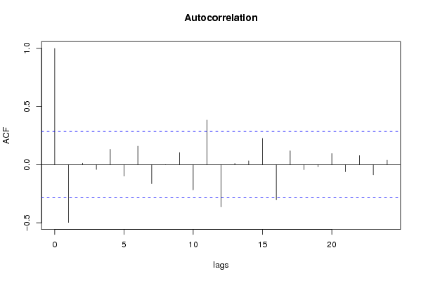
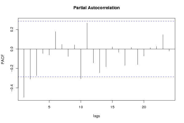
Title produced by software

(Partial) Autocorrelation Function

Date of computation

Sun, 07 Dec 2008 05:59:04 -0700

Cite this page as follows

Statistical Computations at FreeStatistics.org, Office for Research Development and Education, URL https://freestatistics.org/blog/index.php?v=date/2008/Dec/07/t12286547940rqpfudxus47h5j.htm/, Retrieved Sun, 19 May 2024 09:36:41 +0000

Statistical Computations at FreeStatistics.org, Office for Research Development and Education, URL https://freestatistics.org/blog/index.php?pk=29917, Retrieved Sun, 19 May 2024 09:36:41 +0000

QR Codes:

Paste this QR Code to cite your computation.

Original text written by user:

IsPrivate?

No (this computation is public)

User-defined keywords

Estimated Impact

184

Family? (F = Feedback message, R = changed R code, M = changed R Module, P = changed Parameters, D = changed Data)

-     [Standard Deviation-Mean Plot] [Paper Hoofdstuk 4...] [2008-12-05 10:14:55] [6fea0e9a9b3b29a63badf2c274e82506]
- RM D  [Variance Reduction Matrix] [Paper, hoofdstuk ...] [2008-12-06 15:48:43] [79c17183721a40a589db5f9f561947d8]
- RMP     [(Partial) Autocorrelation Function] [Paper, hoofdstuk ...] [2008-12-06 16:56:09] [79c17183721a40a589db5f9f561947d8]
-   P       [(Partial) Autocorrelation Function] [Paper, hoofdstuk ...] [2008-12-06 17:05:19] [79c17183721a40a589db5f9f561947d8]
- RMP         [Spectral Analysis] [Paper, hoofdstuk ...] [2008-12-07 11:35:08] [79c17183721a40a589db5f9f561947d8]
-   P           [Spectral Analysis] [Paper, hoofdstuk ...] [2008-12-07 11:55:02] [79c17183721a40a589db5f9f561947d8]
- RMP               [(Partial) Autocorrelation Function] [Paper, hoofdstuk ...] [2008-12-07 12:59:04] [3bb0537fcae9c337e49b9ce75ff3d4da] [Current]
-   P                 [(Partial) Autocorrelation Function] [Paper, hoofdstuk ...] [2008-12-09 14:22:25] [79c17183721a40a589db5f9f561947d8] 
- RMPD                [ARIMA Backward Selection] [Paper Hoofdstuk 4...] [2008-12-09 14:31:45] [6fea0e9a9b3b29a63badf2c274e82506] 
- RMP                 [ARIMA Backward Selection] [Paper Hoofdstuk 4...] [2008-12-09 14:42:05] [79c17183721a40a589db5f9f561947d8] 
-                       [ARIMA Backward Selection] [Paper, hoofdstuk ...] [2008-12-10 20:45:33] [79c17183721a40a589db5f9f561947d8] 

Feedback Forum

Post a new message

Dataseries X:

Download CSV

Histogram

Boxplots

Summary of computational transaction
Raw Input	view raw input (R code)
Raw Output	view raw output of R engine
Computing time	1 seconds
R Server	'George Udny Yule' @ 72.249.76.132

\begin{tabular}{lllllllll}
\hline
Summary of computational transaction \tabularnewline
Raw Input & view raw input (R code)  \tabularnewline
Raw Output & view raw output of R engine  \tabularnewline
Computing time & 1 seconds \tabularnewline
R Server & 'George Udny Yule' @ 72.249.76.132 \tabularnewline
\hline
\end{tabular}
%Source: https://freestatistics.org/blog/index.php?pk=29917&T=0

[TABLE]
[ROW][C]Summary of computational transaction[/C][/ROW]
[ROW][C]Raw Input[/C][C]view raw input (R code) [/C][/ROW]
[ROW][C]Raw Output[/C][C]view raw output of R engine [/C][/ROW]
[ROW][C]Computing time[/C][C]1 seconds[/C][/ROW]
[ROW][C]R Server[/C][C]'George Udny Yule' @ 72.249.76.132[/C][/ROW]
[/TABLE]
Source: https://freestatistics.org/blog/index.php?pk=29917&T=0

Globally Unique Identifier (entire table): ba.freestatistics.org/blog/index.php?pk=29917&T=0

As an alternative you can also use a QR Code:

The GUIDs for individual cells are displayed in the table below:

Summary of computational transaction
Raw Input	view raw input (R code)
Raw Output	view raw output of R engine
Computing time	1 seconds
R Server	'George Udny Yule' @ 72.249.76.132

Autocorrelation Function
Time lag k	ACF(k)	T-STAT	P-value
1	-0.497375	-3.4098	0.000672
2	0.013555	0.0929	0.463178
3	-0.041367	-0.2836	0.388982
4	0.132207	0.9064	0.184683
5	-0.098484	-0.6752	0.251437
6	0.159188	1.0913	0.140344
7	-0.163734	-1.1225	0.133675
8	-0.001041	-0.0071	0.497167
9	0.104057	0.7134	0.239569
10	-0.216992	-1.4876	0.071765
11	0.383208	2.6271	0.005795
12	-0.364199	-2.4968	0.008047
13	0.011132	0.0763	0.469745
14	0.03256	0.2232	0.412166
15	0.225528	1.5461	0.064389
16	-0.302837	-2.0761	0.021688
17	0.119338	0.8181	0.208703
18	-0.042936	-0.2944	0.384892
19	-0.018365	-0.1259	0.450173
20	0.095699	0.6561	0.257487
21	-0.060518	-0.4149	0.340054
22	0.078	0.5347	0.297674
23	-0.087138	-0.5974	0.276558
24	0.038467	0.2637	0.396574

\begin{tabular}{lllllllll}
\hline
Autocorrelation Function \tabularnewline
Time lag k & ACF(k) & T-STAT & P-value \tabularnewline
1 & -0.497375 & -3.4098 & 0.000672 \tabularnewline
2 & 0.013555 & 0.0929 & 0.463178 \tabularnewline
3 & -0.041367 & -0.2836 & 0.388982 \tabularnewline
4 & 0.132207 & 0.9064 & 0.184683 \tabularnewline
5 & -0.098484 & -0.6752 & 0.251437 \tabularnewline
6 & 0.159188 & 1.0913 & 0.140344 \tabularnewline
7 & -0.163734 & -1.1225 & 0.133675 \tabularnewline
8 & -0.001041 & -0.0071 & 0.497167 \tabularnewline
9 & 0.104057 & 0.7134 & 0.239569 \tabularnewline
10 & -0.216992 & -1.4876 & 0.071765 \tabularnewline
11 & 0.383208 & 2.6271 & 0.005795 \tabularnewline
12 & -0.364199 & -2.4968 & 0.008047 \tabularnewline
13 & 0.011132 & 0.0763 & 0.469745 \tabularnewline
14 & 0.03256 & 0.2232 & 0.412166 \tabularnewline
15 & 0.225528 & 1.5461 & 0.064389 \tabularnewline
16 & -0.302837 & -2.0761 & 0.021688 \tabularnewline
17 & 0.119338 & 0.8181 & 0.208703 \tabularnewline
18 & -0.042936 & -0.2944 & 0.384892 \tabularnewline
19 & -0.018365 & -0.1259 & 0.450173 \tabularnewline
20 & 0.095699 & 0.6561 & 0.257487 \tabularnewline
21 & -0.060518 & -0.4149 & 0.340054 \tabularnewline
22 & 0.078 & 0.5347 & 0.297674 \tabularnewline
23 & -0.087138 & -0.5974 & 0.276558 \tabularnewline
24 & 0.038467 & 0.2637 & 0.396574 \tabularnewline
\hline
\end{tabular}
%Source: https://freestatistics.org/blog/index.php?pk=29917&T=1

[TABLE]
[ROW][C]Autocorrelation Function[/C][/ROW]
[ROW][C]Time lag k[/C][C]ACF(k)[/C][C]T-STAT[/C][C]P-value[/C][/ROW]
[ROW][C]1[/C][C]-0.497375[/C][C]-3.4098[/C][C]0.000672[/C][/ROW]
[ROW][C]2[/C][C]0.013555[/C][C]0.0929[/C][C]0.463178[/C][/ROW]
[ROW][C]3[/C][C]-0.041367[/C][C]-0.2836[/C][C]0.388982[/C][/ROW]
[ROW][C]4[/C][C]0.132207[/C][C]0.9064[/C][C]0.184683[/C][/ROW]
[ROW][C]5[/C][C]-0.098484[/C][C]-0.6752[/C][C]0.251437[/C][/ROW]
[ROW][C]6[/C][C]0.159188[/C][C]1.0913[/C][C]0.140344[/C][/ROW]
[ROW][C]7[/C][C]-0.163734[/C][C]-1.1225[/C][C]0.133675[/C][/ROW]
[ROW][C]8[/C][C]-0.001041[/C][C]-0.0071[/C][C]0.497167[/C][/ROW]
[ROW][C]9[/C][C]0.104057[/C][C]0.7134[/C][C]0.239569[/C][/ROW]
[ROW][C]10[/C][C]-0.216992[/C][C]-1.4876[/C][C]0.071765[/C][/ROW]
[ROW][C]11[/C][C]0.383208[/C][C]2.6271[/C][C]0.005795[/C][/ROW]
[ROW][C]12[/C][C]-0.364199[/C][C]-2.4968[/C][C]0.008047[/C][/ROW]
[ROW][C]13[/C][C]0.011132[/C][C]0.0763[/C][C]0.469745[/C][/ROW]
[ROW][C]14[/C][C]0.03256[/C][C]0.2232[/C][C]0.412166[/C][/ROW]
[ROW][C]15[/C][C]0.225528[/C][C]1.5461[/C][C]0.064389[/C][/ROW]
[ROW][C]16[/C][C]-0.302837[/C][C]-2.0761[/C][C]0.021688[/C][/ROW]
[ROW][C]17[/C][C]0.119338[/C][C]0.8181[/C][C]0.208703[/C][/ROW]
[ROW][C]18[/C][C]-0.042936[/C][C]-0.2944[/C][C]0.384892[/C][/ROW]
[ROW][C]19[/C][C]-0.018365[/C][C]-0.1259[/C][C]0.450173[/C][/ROW]
[ROW][C]20[/C][C]0.095699[/C][C]0.6561[/C][C]0.257487[/C][/ROW]
[ROW][C]21[/C][C]-0.060518[/C][C]-0.4149[/C][C]0.340054[/C][/ROW]
[ROW][C]22[/C][C]0.078[/C][C]0.5347[/C][C]0.297674[/C][/ROW]
[ROW][C]23[/C][C]-0.087138[/C][C]-0.5974[/C][C]0.276558[/C][/ROW]
[ROW][C]24[/C][C]0.038467[/C][C]0.2637[/C][C]0.396574[/C][/ROW]
[/TABLE]
Source: https://freestatistics.org/blog/index.php?pk=29917&T=1

Globally Unique Identifier (entire table): ba.freestatistics.org/blog/index.php?pk=29917&T=1

As an alternative you can also use a QR Code:

The GUIDs for individual cells are displayed in the table below:

Autocorrelation Function
Time lag k	ACF(k)	T-STAT	P-value
1	-0.497375	-3.4098	0.000672
2	0.013555	0.0929	0.463178
3	-0.041367	-0.2836	0.388982
4	0.132207	0.9064	0.184683
5	-0.098484	-0.6752	0.251437
6	0.159188	1.0913	0.140344
7	-0.163734	-1.1225	0.133675
8	-0.001041	-0.0071	0.497167
9	0.104057	0.7134	0.239569
10	-0.216992	-1.4876	0.071765
11	0.383208	2.6271	0.005795
12	-0.364199	-2.4968	0.008047
13	0.011132	0.0763	0.469745
14	0.03256	0.2232	0.412166
15	0.225528	1.5461	0.064389
16	-0.302837	-2.0761	0.021688
17	0.119338	0.8181	0.208703
18	-0.042936	-0.2944	0.384892
19	-0.018365	-0.1259	0.450173
20	0.095699	0.6561	0.257487
21	-0.060518	-0.4149	0.340054
22	0.078	0.5347	0.297674
23	-0.087138	-0.5974	0.276558
24	0.038467	0.2637	0.396574

Partial Autocorrelation Function
Time lag k	PACF(k)	T-STAT	P-value
1	-0.497375	-3.4098	0.000672
2	-0.310685	-2.1299	0.019221
3	-0.275096	-1.886	0.032744
4	-0.045313	-0.3106	0.378721
5	-0.062013	-0.4251	0.336338
6	0.178675	1.2249	0.113352
7	0.047223	0.3237	0.373784
8	-0.076925	-0.5274	0.300208
9	0.042129	0.2888	0.386993
10	-0.306217	-2.0993	0.020593
11	0.266825	1.8293	0.036854
12	-0.143468	-0.9836	0.165182
13	-0.245023	-1.6798	0.049817
14	-0.183321	-1.2568	0.107521
15	0.022331	0.1531	0.43949
16	-0.034034	-0.2333	0.408262
17	-0.168871	-1.1577	0.126414
18	0.016863	0.1156	0.454229
19	-0.160681	-1.1016	0.138129
20	-0.073125	-0.5013	0.309242
21	0.013395	0.0918	0.46361
22	0.025655	0.1759	0.430572
23	0.147489	1.0111	0.158564
24	-0.021458	-0.1471	0.441837

\begin{tabular}{lllllllll}
\hline
Partial Autocorrelation Function \tabularnewline
Time lag k & PACF(k) & T-STAT & P-value \tabularnewline
1 & -0.497375 & -3.4098 & 0.000672 \tabularnewline
2 & -0.310685 & -2.1299 & 0.019221 \tabularnewline
3 & -0.275096 & -1.886 & 0.032744 \tabularnewline
4 & -0.045313 & -0.3106 & 0.378721 \tabularnewline
5 & -0.062013 & -0.4251 & 0.336338 \tabularnewline
6 & 0.178675 & 1.2249 & 0.113352 \tabularnewline
7 & 0.047223 & 0.3237 & 0.373784 \tabularnewline
8 & -0.076925 & -0.5274 & 0.300208 \tabularnewline
9 & 0.042129 & 0.2888 & 0.386993 \tabularnewline
10 & -0.306217 & -2.0993 & 0.020593 \tabularnewline
11 & 0.266825 & 1.8293 & 0.036854 \tabularnewline
12 & -0.143468 & -0.9836 & 0.165182 \tabularnewline
13 & -0.245023 & -1.6798 & 0.049817 \tabularnewline
14 & -0.183321 & -1.2568 & 0.107521 \tabularnewline
15 & 0.022331 & 0.1531 & 0.43949 \tabularnewline
16 & -0.034034 & -0.2333 & 0.408262 \tabularnewline
17 & -0.168871 & -1.1577 & 0.126414 \tabularnewline
18 & 0.016863 & 0.1156 & 0.454229 \tabularnewline
19 & -0.160681 & -1.1016 & 0.138129 \tabularnewline
20 & -0.073125 & -0.5013 & 0.309242 \tabularnewline
21 & 0.013395 & 0.0918 & 0.46361 \tabularnewline
22 & 0.025655 & 0.1759 & 0.430572 \tabularnewline
23 & 0.147489 & 1.0111 & 0.158564 \tabularnewline
24 & -0.021458 & -0.1471 & 0.441837 \tabularnewline
\hline
\end{tabular}
%Source: https://freestatistics.org/blog/index.php?pk=29917&T=2

[TABLE]
[ROW][C]Partial Autocorrelation Function[/C][/ROW]
[ROW][C]Time lag k[/C][C]PACF(k)[/C][C]T-STAT[/C][C]P-value[/C][/ROW]
[ROW][C]1[/C][C]-0.497375[/C][C]-3.4098[/C][C]0.000672[/C][/ROW]
[ROW][C]2[/C][C]-0.310685[/C][C]-2.1299[/C][C]0.019221[/C][/ROW]
[ROW][C]3[/C][C]-0.275096[/C][C]-1.886[/C][C]0.032744[/C][/ROW]
[ROW][C]4[/C][C]-0.045313[/C][C]-0.3106[/C][C]0.378721[/C][/ROW]
[ROW][C]5[/C][C]-0.062013[/C][C]-0.4251[/C][C]0.336338[/C][/ROW]
[ROW][C]6[/C][C]0.178675[/C][C]1.2249[/C][C]0.113352[/C][/ROW]
[ROW][C]7[/C][C]0.047223[/C][C]0.3237[/C][C]0.373784[/C][/ROW]
[ROW][C]8[/C][C]-0.076925[/C][C]-0.5274[/C][C]0.300208[/C][/ROW]
[ROW][C]9[/C][C]0.042129[/C][C]0.2888[/C][C]0.386993[/C][/ROW]
[ROW][C]10[/C][C]-0.306217[/C][C]-2.0993[/C][C]0.020593[/C][/ROW]
[ROW][C]11[/C][C]0.266825[/C][C]1.8293[/C][C]0.036854[/C][/ROW]
[ROW][C]12[/C][C]-0.143468[/C][C]-0.9836[/C][C]0.165182[/C][/ROW]
[ROW][C]13[/C][C]-0.245023[/C][C]-1.6798[/C][C]0.049817[/C][/ROW]
[ROW][C]14[/C][C]-0.183321[/C][C]-1.2568[/C][C]0.107521[/C][/ROW]
[ROW][C]15[/C][C]0.022331[/C][C]0.1531[/C][C]0.43949[/C][/ROW]
[ROW][C]16[/C][C]-0.034034[/C][C]-0.2333[/C][C]0.408262[/C][/ROW]
[ROW][C]17[/C][C]-0.168871[/C][C]-1.1577[/C][C]0.126414[/C][/ROW]
[ROW][C]18[/C][C]0.016863[/C][C]0.1156[/C][C]0.454229[/C][/ROW]
[ROW][C]19[/C][C]-0.160681[/C][C]-1.1016[/C][C]0.138129[/C][/ROW]
[ROW][C]20[/C][C]-0.073125[/C][C]-0.5013[/C][C]0.309242[/C][/ROW]
[ROW][C]21[/C][C]0.013395[/C][C]0.0918[/C][C]0.46361[/C][/ROW]
[ROW][C]22[/C][C]0.025655[/C][C]0.1759[/C][C]0.430572[/C][/ROW]
[ROW][C]23[/C][C]0.147489[/C][C]1.0111[/C][C]0.158564[/C][/ROW]
[ROW][C]24[/C][C]-0.021458[/C][C]-0.1471[/C][C]0.441837[/C][/ROW]
[/TABLE]
Source: https://freestatistics.org/blog/index.php?pk=29917&T=2

Globally Unique Identifier (entire table): ba.freestatistics.org/blog/index.php?pk=29917&T=2

As an alternative you can also use a QR Code:

The GUIDs for individual cells are displayed in the table below:

Partial Autocorrelation Function
Time lag k	PACF(k)	T-STAT	P-value
1	-0.497375	-3.4098	0.000672
2	-0.310685	-2.1299	0.019221
3	-0.275096	-1.886	0.032744
4	-0.045313	-0.3106	0.378721
5	-0.062013	-0.4251	0.336338
6	0.178675	1.2249	0.113352
7	0.047223	0.3237	0.373784
8	-0.076925	-0.5274	0.300208
9	0.042129	0.2888	0.386993
10	-0.306217	-2.0993	0.020593
11	0.266825	1.8293	0.036854
12	-0.143468	-0.9836	0.165182
13	-0.245023	-1.6798	0.049817
14	-0.183321	-1.2568	0.107521
15	0.022331	0.1531	0.43949
16	-0.034034	-0.2333	0.408262
17	-0.168871	-1.1577	0.126414
18	0.016863	0.1156	0.454229
19	-0.160681	-1.1016	0.138129
20	-0.073125	-0.5013	0.309242
21	0.013395	0.0918	0.46361
22	0.025655	0.1759	0.430572
23	0.147489	1.0111	0.158564
24	-0.021458	-0.1471	0.441837

Figure 1

PNG link

Postscript link

PDF link

Figure 2

PNG link

Postscript link

PDF link

Parameters (Session):

par1 = 24 ; par2 = -1.7 ; par3 = 1 ; par4 = 1 ; par5 = 12 ;

Parameters (R input):

par1 = 24 ; par2 = -1.7 ; par3 = 1 ; par4 = 1 ; par5 = 12 ;

R code (references can be found in the software module):

if (par1 == 'Default') {
par1 = 10*log10(length(x))
} else {
par1 <- as.numeric(par1)
}
par2 <- as.numeric(par2)
par3 <- as.numeric(par3)
par4 <- as.numeric(par4)
par5 <- as.numeric(par5)
if (par2 == 0) {
x <- log(x)
} else {
x <- (x ^ par2 - 1) / par2
}
if (par3 > 0) x <- diff(x,lag=1,difference=par3)
if (par4 > 0) x <- diff(x,lag=par5,difference=par4)
bitmap(file='pic1.png')
racf <- acf(x,par1,main='Autocorrelation',xlab='lags',ylab='ACF')
dev.off()
bitmap(file='pic2.png')
rpacf <- pacf(x,par1,main='Partial Autocorrelation',xlab='lags',ylab='PACF')
dev.off()
(myacf <- c(racf$acf))
(mypacf <- c(rpacf$acf))
lengthx <- length(x)
sqrtn <- sqrt(lengthx)
load(file='createtable')
a<-table.start()
a<-table.row.start(a)
a<-table.element(a,'Autocorrelation Function',4,TRUE)
a<-table.row.end(a)
a<-table.row.start(a)
a<-table.element(a,'Time lag k',header=TRUE)
a<-table.element(a,hyperlink('basics.htm','ACF(k)','click here for more information about the Autocorrelation Function'),header=TRUE)
a<-table.element(a,'T-STAT',header=TRUE)
a<-table.element(a,'P-value',header=TRUE)
a<-table.row.end(a)
for (i in 2:(par1+1)) {
a<-table.row.start(a)
a<-table.element(a,i-1,header=TRUE)
a<-table.element(a,round(myacf[i],6))
mytstat <- myacf[i]*sqrtn
a<-table.element(a,round(mytstat,4))
a<-table.element(a,round(1-pt(abs(mytstat),lengthx),6))
a<-table.row.end(a)
}
a<-table.end(a)
table.save(a,file='mytable.tab')
a<-table.start()
a<-table.row.start(a)
a<-table.element(a,'Partial Autocorrelation Function',4,TRUE)
a<-table.row.end(a)
a<-table.row.start(a)
a<-table.element(a,'Time lag k',header=TRUE)
a<-table.element(a,hyperlink('basics.htm','PACF(k)','click here for more information about the Partial Autocorrelation Function'),header=TRUE)
a<-table.element(a,'T-STAT',header=TRUE)
a<-table.element(a,'P-value',header=TRUE)
a<-table.row.end(a)
for (i in 1:par1) {
a<-table.row.start(a)
a<-table.element(a,i,header=TRUE)
a<-table.element(a,round(mypacf[i],6))
mytstat <- mypacf[i]*sqrtn
a<-table.element(a,round(mytstat,4))
a<-table.element(a,round(1-pt(abs(mytstat),lengthx),6))
a<-table.row.end(a)
}
a<-table.end(a)
table.save(a,file='mytable1.tab')

Free Statistics

Description of Statistical Computation

Tree of Dependent Computations

Dataset

Tables (Output of Computation)

Figures (Output of Computation)

Input Parameters & R Code