Repository of Reproducible Computations

Free Statistics

of Irreproducible Research!

Author's title

Author

*The author of this computation has been verified*

R Software Module

rwasp_autocorrelation.wasp

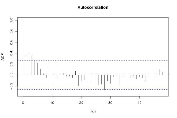
Title produced by software

(Partial) Autocorrelation Function

Date of computation

Sat, 06 Dec 2008 11:25:21 -0700

Cite this page as follows

Statistical Computations at FreeStatistics.org, Office for Research Development and Education, URL https://freestatistics.org/blog/index.php?v=date/2008/Dec/06/t1228587959pd6l92dvruem7ja.htm/, Retrieved Sun, 19 May 2024 11:31:42 +0000

Statistical Computations at FreeStatistics.org, Office for Research Development and Education, URL https://freestatistics.org/blog/index.php?pk=29795, Retrieved Sun, 19 May 2024 11:31:42 +0000

QR Codes:

Paste this QR Code to cite your computation.

Original text written by user:

IsPrivate?

No (this computation is public)

User-defined keywords

Estimated Impact

184

Family? (F = Feedback message, R = changed R code, M = changed R Module, P = changed Parameters, D = changed Data)

-     [Univariate Data Series] [data set] [2008-12-01 19:54:57] [b98453cac15ba1066b407e146608df68]
-   P   [Univariate Data Series] [Werkloosheid] [2008-12-06 16:45:11] [b82ef11dce0545f3fd4676ec3ebed828]
- RMP     [Standard Deviation-Mean Plot] [Identification an...] [2008-12-06 17:10:24] [b82ef11dce0545f3fd4676ec3ebed828]
-   P       [Standard Deviation-Mean Plot] [Identification an...] [2008-12-06 17:29:58] [b82ef11dce0545f3fd4676ec3ebed828]
- RM          [Variance Reduction Matrix] [Identification an...] [2008-12-06 18:03:38] [b82ef11dce0545f3fd4676ec3ebed828]
-    D          [Variance Reduction Matrix] [Identification an...] [2008-12-06 18:06:13] [b82ef11dce0545f3fd4676ec3ebed828]
- RMP               [(Partial) Autocorrelation Function] [Identification an...] [2008-12-06 18:25:21] [4b953869c7238aca4b6e0cfb0c5cddd6] [Current]
- RMP                 [Spectral Analysis] [Identification an...] [2008-12-06 18:48:08] [b82ef11dce0545f3fd4676ec3ebed828] 

Feedback Forum

Post a new message

Dataseries X:

Download CSV

Histogram

Boxplots

Summary of computational transaction
Raw Input	view raw input (R code)
Raw Output	view raw output of R engine
Computing time	1 seconds
R Server	'George Udny Yule' @ 72.249.76.132

\begin{tabular}{lllllllll}
\hline
Summary of computational transaction \tabularnewline
Raw Input & view raw input (R code)  \tabularnewline
Raw Output & view raw output of R engine  \tabularnewline
Computing time & 1 seconds \tabularnewline
R Server & 'George Udny Yule' @ 72.249.76.132 \tabularnewline
\hline
\end{tabular}
%Source: https://freestatistics.org/blog/index.php?pk=29795&T=0

[TABLE]
[ROW][C]Summary of computational transaction[/C][/ROW]
[ROW][C]Raw Input[/C][C]view raw input (R code) [/C][/ROW]
[ROW][C]Raw Output[/C][C]view raw output of R engine [/C][/ROW]
[ROW][C]Computing time[/C][C]1 seconds[/C][/ROW]
[ROW][C]R Server[/C][C]'George Udny Yule' @ 72.249.76.132[/C][/ROW]
[/TABLE]
Source: https://freestatistics.org/blog/index.php?pk=29795&T=0

Globally Unique Identifier (entire table): ba.freestatistics.org/blog/index.php?pk=29795&T=0

As an alternative you can also use a QR Code:

The GUIDs for individual cells are displayed in the table below:

Summary of computational transaction
Raw Input	view raw input (R code)
Raw Output	view raw output of R engine
Computing time	1 seconds
R Server	'George Udny Yule' @ 72.249.76.132

Autocorrelation Function
Time lag k	ACF(k)	T-STAT	P-value
1	0.359016	2.6625	0.005075
2	0.410017	3.0408	0.001805
3	0.353978	2.6252	0.005596
4	0.260116	1.9291	0.029444
5	0.225066	1.6691	0.050387
6	0.114459	0.8489	0.199822
7	0.027255	0.2021	0.420282
8	-0.043525	-0.3228	0.37404
9	0.138701	1.0286	0.154077
10	-0.15232	-1.1296	0.131766
11	-0.032302	-0.2396	0.405781
12	-0.072539	-0.538	0.296386
13	0.023953	0.1776	0.429828
14	0.037289	0.2765	0.391583
15	-0.020476	-0.1519	0.439928
16	-0.010663	-0.0791	0.468628
17	-0.047568	-0.3528	0.362804
18	0.072708	0.5392	0.295956
19	-0.19244	-1.4272	0.079592
20	-0.099577	-0.7385	0.231681
21	-0.089061	-0.6605	0.255848
22	-0.188343	-1.3968	0.084044
23	-0.123179	-0.9135	0.182479
24	-0.333885	-2.4762	0.008193
25	-0.260053	-1.9286	0.029474
26	-0.176321	-1.3076	0.098219
27	-0.166502	-1.2348	0.111075
28	-0.273305	-2.0269	0.023767
29	-0.108346	-0.8035	0.212568
30	-0.154225	-1.1438	0.128837
31	-0.028283	-0.2098	0.417318
32	-0.004987	-0.037	0.485315
33	-0.177941	-1.3196	0.09621
34	-0.040737	-0.3021	0.381851
35	-0.038642	-0.2866	0.387758
36	-0.027502	-0.204	0.419569
37	-0.046984	-0.3484	0.364419
38	-0.021009	-0.1558	0.438378
39	-0.074212	-0.5504	0.292146
40	-0.028205	-0.2092	0.417544
41	-0.050175	-0.3721	0.35562
42	-0.108558	-0.8051	0.212118
43	-0.044273	-0.3283	0.371953
44	0.035096	0.2603	0.397809
45	-0.012673	-0.094	0.46273
46	0.042386	0.3143	0.377225
47	0.103782	0.7697	0.222395
48	0.059764	0.4432	0.329671

\begin{tabular}{lllllllll}
\hline
Autocorrelation Function \tabularnewline
Time lag k & ACF(k) & T-STAT & P-value \tabularnewline
1 & 0.359016 & 2.6625 & 0.005075 \tabularnewline
2 & 0.410017 & 3.0408 & 0.001805 \tabularnewline
3 & 0.353978 & 2.6252 & 0.005596 \tabularnewline
4 & 0.260116 & 1.9291 & 0.029444 \tabularnewline
5 & 0.225066 & 1.6691 & 0.050387 \tabularnewline
6 & 0.114459 & 0.8489 & 0.199822 \tabularnewline
7 & 0.027255 & 0.2021 & 0.420282 \tabularnewline
8 & -0.043525 & -0.3228 & 0.37404 \tabularnewline
9 & 0.138701 & 1.0286 & 0.154077 \tabularnewline
10 & -0.15232 & -1.1296 & 0.131766 \tabularnewline
11 & -0.032302 & -0.2396 & 0.405781 \tabularnewline
12 & -0.072539 & -0.538 & 0.296386 \tabularnewline
13 & 0.023953 & 0.1776 & 0.429828 \tabularnewline
14 & 0.037289 & 0.2765 & 0.391583 \tabularnewline
15 & -0.020476 & -0.1519 & 0.439928 \tabularnewline
16 & -0.010663 & -0.0791 & 0.468628 \tabularnewline
17 & -0.047568 & -0.3528 & 0.362804 \tabularnewline
18 & 0.072708 & 0.5392 & 0.295956 \tabularnewline
19 & -0.19244 & -1.4272 & 0.079592 \tabularnewline
20 & -0.099577 & -0.7385 & 0.231681 \tabularnewline
21 & -0.089061 & -0.6605 & 0.255848 \tabularnewline
22 & -0.188343 & -1.3968 & 0.084044 \tabularnewline
23 & -0.123179 & -0.9135 & 0.182479 \tabularnewline
24 & -0.333885 & -2.4762 & 0.008193 \tabularnewline
25 & -0.260053 & -1.9286 & 0.029474 \tabularnewline
26 & -0.176321 & -1.3076 & 0.098219 \tabularnewline
27 & -0.166502 & -1.2348 & 0.111075 \tabularnewline
28 & -0.273305 & -2.0269 & 0.023767 \tabularnewline
29 & -0.108346 & -0.8035 & 0.212568 \tabularnewline
30 & -0.154225 & -1.1438 & 0.128837 \tabularnewline
31 & -0.028283 & -0.2098 & 0.417318 \tabularnewline
32 & -0.004987 & -0.037 & 0.485315 \tabularnewline
33 & -0.177941 & -1.3196 & 0.09621 \tabularnewline
34 & -0.040737 & -0.3021 & 0.381851 \tabularnewline
35 & -0.038642 & -0.2866 & 0.387758 \tabularnewline
36 & -0.027502 & -0.204 & 0.419569 \tabularnewline
37 & -0.046984 & -0.3484 & 0.364419 \tabularnewline
38 & -0.021009 & -0.1558 & 0.438378 \tabularnewline
39 & -0.074212 & -0.5504 & 0.292146 \tabularnewline
40 & -0.028205 & -0.2092 & 0.417544 \tabularnewline
41 & -0.050175 & -0.3721 & 0.35562 \tabularnewline
42 & -0.108558 & -0.8051 & 0.212118 \tabularnewline
43 & -0.044273 & -0.3283 & 0.371953 \tabularnewline
44 & 0.035096 & 0.2603 & 0.397809 \tabularnewline
45 & -0.012673 & -0.094 & 0.46273 \tabularnewline
46 & 0.042386 & 0.3143 & 0.377225 \tabularnewline
47 & 0.103782 & 0.7697 & 0.222395 \tabularnewline
48 & 0.059764 & 0.4432 & 0.329671 \tabularnewline
\hline
\end{tabular}
%Source: https://freestatistics.org/blog/index.php?pk=29795&T=1

[TABLE]
[ROW][C]Autocorrelation Function[/C][/ROW]
[ROW][C]Time lag k[/C][C]ACF(k)[/C][C]T-STAT[/C][C]P-value[/C][/ROW]
[ROW][C]1[/C][C]0.359016[/C][C]2.6625[/C][C]0.005075[/C][/ROW]
[ROW][C]2[/C][C]0.410017[/C][C]3.0408[/C][C]0.001805[/C][/ROW]
[ROW][C]3[/C][C]0.353978[/C][C]2.6252[/C][C]0.005596[/C][/ROW]
[ROW][C]4[/C][C]0.260116[/C][C]1.9291[/C][C]0.029444[/C][/ROW]
[ROW][C]5[/C][C]0.225066[/C][C]1.6691[/C][C]0.050387[/C][/ROW]
[ROW][C]6[/C][C]0.114459[/C][C]0.8489[/C][C]0.199822[/C][/ROW]
[ROW][C]7[/C][C]0.027255[/C][C]0.2021[/C][C]0.420282[/C][/ROW]
[ROW][C]8[/C][C]-0.043525[/C][C]-0.3228[/C][C]0.37404[/C][/ROW]
[ROW][C]9[/C][C]0.138701[/C][C]1.0286[/C][C]0.154077[/C][/ROW]
[ROW][C]10[/C][C]-0.15232[/C][C]-1.1296[/C][C]0.131766[/C][/ROW]
[ROW][C]11[/C][C]-0.032302[/C][C]-0.2396[/C][C]0.405781[/C][/ROW]
[ROW][C]12[/C][C]-0.072539[/C][C]-0.538[/C][C]0.296386[/C][/ROW]
[ROW][C]13[/C][C]0.023953[/C][C]0.1776[/C][C]0.429828[/C][/ROW]
[ROW][C]14[/C][C]0.037289[/C][C]0.2765[/C][C]0.391583[/C][/ROW]
[ROW][C]15[/C][C]-0.020476[/C][C]-0.1519[/C][C]0.439928[/C][/ROW]
[ROW][C]16[/C][C]-0.010663[/C][C]-0.0791[/C][C]0.468628[/C][/ROW]
[ROW][C]17[/C][C]-0.047568[/C][C]-0.3528[/C][C]0.362804[/C][/ROW]
[ROW][C]18[/C][C]0.072708[/C][C]0.5392[/C][C]0.295956[/C][/ROW]
[ROW][C]19[/C][C]-0.19244[/C][C]-1.4272[/C][C]0.079592[/C][/ROW]
[ROW][C]20[/C][C]-0.099577[/C][C]-0.7385[/C][C]0.231681[/C][/ROW]
[ROW][C]21[/C][C]-0.089061[/C][C]-0.6605[/C][C]0.255848[/C][/ROW]
[ROW][C]22[/C][C]-0.188343[/C][C]-1.3968[/C][C]0.084044[/C][/ROW]
[ROW][C]23[/C][C]-0.123179[/C][C]-0.9135[/C][C]0.182479[/C][/ROW]
[ROW][C]24[/C][C]-0.333885[/C][C]-2.4762[/C][C]0.008193[/C][/ROW]
[ROW][C]25[/C][C]-0.260053[/C][C]-1.9286[/C][C]0.029474[/C][/ROW]
[ROW][C]26[/C][C]-0.176321[/C][C]-1.3076[/C][C]0.098219[/C][/ROW]
[ROW][C]27[/C][C]-0.166502[/C][C]-1.2348[/C][C]0.111075[/C][/ROW]
[ROW][C]28[/C][C]-0.273305[/C][C]-2.0269[/C][C]0.023767[/C][/ROW]
[ROW][C]29[/C][C]-0.108346[/C][C]-0.8035[/C][C]0.212568[/C][/ROW]
[ROW][C]30[/C][C]-0.154225[/C][C]-1.1438[/C][C]0.128837[/C][/ROW]
[ROW][C]31[/C][C]-0.028283[/C][C]-0.2098[/C][C]0.417318[/C][/ROW]
[ROW][C]32[/C][C]-0.004987[/C][C]-0.037[/C][C]0.485315[/C][/ROW]
[ROW][C]33[/C][C]-0.177941[/C][C]-1.3196[/C][C]0.09621[/C][/ROW]
[ROW][C]34[/C][C]-0.040737[/C][C]-0.3021[/C][C]0.381851[/C][/ROW]
[ROW][C]35[/C][C]-0.038642[/C][C]-0.2866[/C][C]0.387758[/C][/ROW]
[ROW][C]36[/C][C]-0.027502[/C][C]-0.204[/C][C]0.419569[/C][/ROW]
[ROW][C]37[/C][C]-0.046984[/C][C]-0.3484[/C][C]0.364419[/C][/ROW]
[ROW][C]38[/C][C]-0.021009[/C][C]-0.1558[/C][C]0.438378[/C][/ROW]
[ROW][C]39[/C][C]-0.074212[/C][C]-0.5504[/C][C]0.292146[/C][/ROW]
[ROW][C]40[/C][C]-0.028205[/C][C]-0.2092[/C][C]0.417544[/C][/ROW]
[ROW][C]41[/C][C]-0.050175[/C][C]-0.3721[/C][C]0.35562[/C][/ROW]
[ROW][C]42[/C][C]-0.108558[/C][C]-0.8051[/C][C]0.212118[/C][/ROW]
[ROW][C]43[/C][C]-0.044273[/C][C]-0.3283[/C][C]0.371953[/C][/ROW]
[ROW][C]44[/C][C]0.035096[/C][C]0.2603[/C][C]0.397809[/C][/ROW]
[ROW][C]45[/C][C]-0.012673[/C][C]-0.094[/C][C]0.46273[/C][/ROW]
[ROW][C]46[/C][C]0.042386[/C][C]0.3143[/C][C]0.377225[/C][/ROW]
[ROW][C]47[/C][C]0.103782[/C][C]0.7697[/C][C]0.222395[/C][/ROW]
[ROW][C]48[/C][C]0.059764[/C][C]0.4432[/C][C]0.329671[/C][/ROW]
[/TABLE]
Source: https://freestatistics.org/blog/index.php?pk=29795&T=1

Globally Unique Identifier (entire table): ba.freestatistics.org/blog/index.php?pk=29795&T=1

As an alternative you can also use a QR Code:

The GUIDs for individual cells are displayed in the table below:

Autocorrelation Function
Time lag k	ACF(k)	T-STAT	P-value
1	0.359016	2.6625	0.005075
2	0.410017	3.0408	0.001805
3	0.353978	2.6252	0.005596
4	0.260116	1.9291	0.029444
5	0.225066	1.6691	0.050387
6	0.114459	0.8489	0.199822
7	0.027255	0.2021	0.420282
8	-0.043525	-0.3228	0.37404
9	0.138701	1.0286	0.154077
10	-0.15232	-1.1296	0.131766
11	-0.032302	-0.2396	0.405781
12	-0.072539	-0.538	0.296386
13	0.023953	0.1776	0.429828
14	0.037289	0.2765	0.391583
15	-0.020476	-0.1519	0.439928
16	-0.010663	-0.0791	0.468628
17	-0.047568	-0.3528	0.362804
18	0.072708	0.5392	0.295956
19	-0.19244	-1.4272	0.079592
20	-0.099577	-0.7385	0.231681
21	-0.089061	-0.6605	0.255848
22	-0.188343	-1.3968	0.084044
23	-0.123179	-0.9135	0.182479
24	-0.333885	-2.4762	0.008193
25	-0.260053	-1.9286	0.029474
26	-0.176321	-1.3076	0.098219
27	-0.166502	-1.2348	0.111075
28	-0.273305	-2.0269	0.023767
29	-0.108346	-0.8035	0.212568
30	-0.154225	-1.1438	0.128837
31	-0.028283	-0.2098	0.417318
32	-0.004987	-0.037	0.485315
33	-0.177941	-1.3196	0.09621
34	-0.040737	-0.3021	0.381851
35	-0.038642	-0.2866	0.387758
36	-0.027502	-0.204	0.419569
37	-0.046984	-0.3484	0.364419
38	-0.021009	-0.1558	0.438378
39	-0.074212	-0.5504	0.292146
40	-0.028205	-0.2092	0.417544
41	-0.050175	-0.3721	0.35562
42	-0.108558	-0.8051	0.212118
43	-0.044273	-0.3283	0.371953
44	0.035096	0.2603	0.397809
45	-0.012673	-0.094	0.46273
46	0.042386	0.3143	0.377225
47	0.103782	0.7697	0.222395
48	0.059764	0.4432	0.329671

Partial Autocorrelation Function
Time lag k	PACF(k)	T-STAT	P-value
1	0.359016	2.6625	0.005075
2	0.322721	2.3934	0.010067
3	0.177373	1.3154	0.096911
4	0.021155	0.1569	0.437952
5	0.002779	0.0206	0.491817
6	-0.090242	-0.6693	0.253066
7	-0.128125	-0.9502	0.173084
8	-0.118768	-0.8808	0.191128
9	0.242754	1.8003	0.038648
10	-0.191277	-1.4186	0.080836
11	0.007995	0.0593	0.476467
12	-0.009131	-0.0677	0.473128
13	0.163858	1.2152	0.11474
14	0.042996	0.3189	0.375516
15	-0.050004	-0.3708	0.35609
16	-0.05623	-0.417	0.339147
17	-0.074685	-0.5539	0.290953
18	0.021604	0.1602	0.436647
19	-0.208159	-1.5437	0.064192
20	-0.063238	-0.469	0.320467
21	0.110263	0.8177	0.20852
22	-0.145824	-1.0815	0.142106
23	0.018242	0.1353	0.446439
24	-0.254006	-1.8838	0.032444
25	-0.016186	-0.12	0.452446
26	0.111327	0.8256	0.206293
27	-0.043452	-0.3222	0.374243
28	-0.050356	-0.3734	0.355126
29	0.04346	0.3223	0.374221
30	-0.072668	-0.5389	0.296058
31	0.125393	0.9299	0.178233
32	-0.056936	-0.4222	0.337246
33	-0.101691	-0.7542	0.226985
34	-0.103185	-0.7652	0.223699
35	-0.013835	-0.1026	0.459325
36	-0.014077	-0.1044	0.458618
37	0.141791	1.0515	0.148802
38	-0.001216	-0.009	0.496418
39	-0.088183	-0.654	0.257925
40	-0.067516	-0.5007	0.309286
41	-0.069738	-0.5172	0.303548
42	0.010396	0.0771	0.469412
43	-0.041009	-0.3041	0.381087
44	0.023922	0.1774	0.429918
45	0.027943	0.2072	0.418298
46	0.038024	0.282	0.389503
47	0.057318	0.4251	0.336217
48	-0.034581	-0.2565	0.399276

\begin{tabular}{lllllllll}
\hline
Partial Autocorrelation Function \tabularnewline
Time lag k & PACF(k) & T-STAT & P-value \tabularnewline
1 & 0.359016 & 2.6625 & 0.005075 \tabularnewline
2 & 0.322721 & 2.3934 & 0.010067 \tabularnewline
3 & 0.177373 & 1.3154 & 0.096911 \tabularnewline
4 & 0.021155 & 0.1569 & 0.437952 \tabularnewline
5 & 0.002779 & 0.0206 & 0.491817 \tabularnewline
6 & -0.090242 & -0.6693 & 0.253066 \tabularnewline
7 & -0.128125 & -0.9502 & 0.173084 \tabularnewline
8 & -0.118768 & -0.8808 & 0.191128 \tabularnewline
9 & 0.242754 & 1.8003 & 0.038648 \tabularnewline
10 & -0.191277 & -1.4186 & 0.080836 \tabularnewline
11 & 0.007995 & 0.0593 & 0.476467 \tabularnewline
12 & -0.009131 & -0.0677 & 0.473128 \tabularnewline
13 & 0.163858 & 1.2152 & 0.11474 \tabularnewline
14 & 0.042996 & 0.3189 & 0.375516 \tabularnewline
15 & -0.050004 & -0.3708 & 0.35609 \tabularnewline
16 & -0.05623 & -0.417 & 0.339147 \tabularnewline
17 & -0.074685 & -0.5539 & 0.290953 \tabularnewline
18 & 0.021604 & 0.1602 & 0.436647 \tabularnewline
19 & -0.208159 & -1.5437 & 0.064192 \tabularnewline
20 & -0.063238 & -0.469 & 0.320467 \tabularnewline
21 & 0.110263 & 0.8177 & 0.20852 \tabularnewline
22 & -0.145824 & -1.0815 & 0.142106 \tabularnewline
23 & 0.018242 & 0.1353 & 0.446439 \tabularnewline
24 & -0.254006 & -1.8838 & 0.032444 \tabularnewline
25 & -0.016186 & -0.12 & 0.452446 \tabularnewline
26 & 0.111327 & 0.8256 & 0.206293 \tabularnewline
27 & -0.043452 & -0.3222 & 0.374243 \tabularnewline
28 & -0.050356 & -0.3734 & 0.355126 \tabularnewline
29 & 0.04346 & 0.3223 & 0.374221 \tabularnewline
30 & -0.072668 & -0.5389 & 0.296058 \tabularnewline
31 & 0.125393 & 0.9299 & 0.178233 \tabularnewline
32 & -0.056936 & -0.4222 & 0.337246 \tabularnewline
33 & -0.101691 & -0.7542 & 0.226985 \tabularnewline
34 & -0.103185 & -0.7652 & 0.223699 \tabularnewline
35 & -0.013835 & -0.1026 & 0.459325 \tabularnewline
36 & -0.014077 & -0.1044 & 0.458618 \tabularnewline
37 & 0.141791 & 1.0515 & 0.148802 \tabularnewline
38 & -0.001216 & -0.009 & 0.496418 \tabularnewline
39 & -0.088183 & -0.654 & 0.257925 \tabularnewline
40 & -0.067516 & -0.5007 & 0.309286 \tabularnewline
41 & -0.069738 & -0.5172 & 0.303548 \tabularnewline
42 & 0.010396 & 0.0771 & 0.469412 \tabularnewline
43 & -0.041009 & -0.3041 & 0.381087 \tabularnewline
44 & 0.023922 & 0.1774 & 0.429918 \tabularnewline
45 & 0.027943 & 0.2072 & 0.418298 \tabularnewline
46 & 0.038024 & 0.282 & 0.389503 \tabularnewline
47 & 0.057318 & 0.4251 & 0.336217 \tabularnewline
48 & -0.034581 & -0.2565 & 0.399276 \tabularnewline
\hline
\end{tabular}
%Source: https://freestatistics.org/blog/index.php?pk=29795&T=2

[TABLE]
[ROW][C]Partial Autocorrelation Function[/C][/ROW]
[ROW][C]Time lag k[/C][C]PACF(k)[/C][C]T-STAT[/C][C]P-value[/C][/ROW]
[ROW][C]1[/C][C]0.359016[/C][C]2.6625[/C][C]0.005075[/C][/ROW]
[ROW][C]2[/C][C]0.322721[/C][C]2.3934[/C][C]0.010067[/C][/ROW]
[ROW][C]3[/C][C]0.177373[/C][C]1.3154[/C][C]0.096911[/C][/ROW]
[ROW][C]4[/C][C]0.021155[/C][C]0.1569[/C][C]0.437952[/C][/ROW]
[ROW][C]5[/C][C]0.002779[/C][C]0.0206[/C][C]0.491817[/C][/ROW]
[ROW][C]6[/C][C]-0.090242[/C][C]-0.6693[/C][C]0.253066[/C][/ROW]
[ROW][C]7[/C][C]-0.128125[/C][C]-0.9502[/C][C]0.173084[/C][/ROW]
[ROW][C]8[/C][C]-0.118768[/C][C]-0.8808[/C][C]0.191128[/C][/ROW]
[ROW][C]9[/C][C]0.242754[/C][C]1.8003[/C][C]0.038648[/C][/ROW]
[ROW][C]10[/C][C]-0.191277[/C][C]-1.4186[/C][C]0.080836[/C][/ROW]
[ROW][C]11[/C][C]0.007995[/C][C]0.0593[/C][C]0.476467[/C][/ROW]
[ROW][C]12[/C][C]-0.009131[/C][C]-0.0677[/C][C]0.473128[/C][/ROW]
[ROW][C]13[/C][C]0.163858[/C][C]1.2152[/C][C]0.11474[/C][/ROW]
[ROW][C]14[/C][C]0.042996[/C][C]0.3189[/C][C]0.375516[/C][/ROW]
[ROW][C]15[/C][C]-0.050004[/C][C]-0.3708[/C][C]0.35609[/C][/ROW]
[ROW][C]16[/C][C]-0.05623[/C][C]-0.417[/C][C]0.339147[/C][/ROW]
[ROW][C]17[/C][C]-0.074685[/C][C]-0.5539[/C][C]0.290953[/C][/ROW]
[ROW][C]18[/C][C]0.021604[/C][C]0.1602[/C][C]0.436647[/C][/ROW]
[ROW][C]19[/C][C]-0.208159[/C][C]-1.5437[/C][C]0.064192[/C][/ROW]
[ROW][C]20[/C][C]-0.063238[/C][C]-0.469[/C][C]0.320467[/C][/ROW]
[ROW][C]21[/C][C]0.110263[/C][C]0.8177[/C][C]0.20852[/C][/ROW]
[ROW][C]22[/C][C]-0.145824[/C][C]-1.0815[/C][C]0.142106[/C][/ROW]
[ROW][C]23[/C][C]0.018242[/C][C]0.1353[/C][C]0.446439[/C][/ROW]
[ROW][C]24[/C][C]-0.254006[/C][C]-1.8838[/C][C]0.032444[/C][/ROW]
[ROW][C]25[/C][C]-0.016186[/C][C]-0.12[/C][C]0.452446[/C][/ROW]
[ROW][C]26[/C][C]0.111327[/C][C]0.8256[/C][C]0.206293[/C][/ROW]
[ROW][C]27[/C][C]-0.043452[/C][C]-0.3222[/C][C]0.374243[/C][/ROW]
[ROW][C]28[/C][C]-0.050356[/C][C]-0.3734[/C][C]0.355126[/C][/ROW]
[ROW][C]29[/C][C]0.04346[/C][C]0.3223[/C][C]0.374221[/C][/ROW]
[ROW][C]30[/C][C]-0.072668[/C][C]-0.5389[/C][C]0.296058[/C][/ROW]
[ROW][C]31[/C][C]0.125393[/C][C]0.9299[/C][C]0.178233[/C][/ROW]
[ROW][C]32[/C][C]-0.056936[/C][C]-0.4222[/C][C]0.337246[/C][/ROW]
[ROW][C]33[/C][C]-0.101691[/C][C]-0.7542[/C][C]0.226985[/C][/ROW]
[ROW][C]34[/C][C]-0.103185[/C][C]-0.7652[/C][C]0.223699[/C][/ROW]
[ROW][C]35[/C][C]-0.013835[/C][C]-0.1026[/C][C]0.459325[/C][/ROW]
[ROW][C]36[/C][C]-0.014077[/C][C]-0.1044[/C][C]0.458618[/C][/ROW]
[ROW][C]37[/C][C]0.141791[/C][C]1.0515[/C][C]0.148802[/C][/ROW]
[ROW][C]38[/C][C]-0.001216[/C][C]-0.009[/C][C]0.496418[/C][/ROW]
[ROW][C]39[/C][C]-0.088183[/C][C]-0.654[/C][C]0.257925[/C][/ROW]
[ROW][C]40[/C][C]-0.067516[/C][C]-0.5007[/C][C]0.309286[/C][/ROW]
[ROW][C]41[/C][C]-0.069738[/C][C]-0.5172[/C][C]0.303548[/C][/ROW]
[ROW][C]42[/C][C]0.010396[/C][C]0.0771[/C][C]0.469412[/C][/ROW]
[ROW][C]43[/C][C]-0.041009[/C][C]-0.3041[/C][C]0.381087[/C][/ROW]
[ROW][C]44[/C][C]0.023922[/C][C]0.1774[/C][C]0.429918[/C][/ROW]
[ROW][C]45[/C][C]0.027943[/C][C]0.2072[/C][C]0.418298[/C][/ROW]
[ROW][C]46[/C][C]0.038024[/C][C]0.282[/C][C]0.389503[/C][/ROW]
[ROW][C]47[/C][C]0.057318[/C][C]0.4251[/C][C]0.336217[/C][/ROW]
[ROW][C]48[/C][C]-0.034581[/C][C]-0.2565[/C][C]0.399276[/C][/ROW]
[/TABLE]
Source: https://freestatistics.org/blog/index.php?pk=29795&T=2

Globally Unique Identifier (entire table): ba.freestatistics.org/blog/index.php?pk=29795&T=2

As an alternative you can also use a QR Code:

The GUIDs for individual cells are displayed in the table below:

Partial Autocorrelation Function
Time lag k	PACF(k)	T-STAT	P-value
1	0.359016	2.6625	0.005075
2	0.322721	2.3934	0.010067
3	0.177373	1.3154	0.096911
4	0.021155	0.1569	0.437952
5	0.002779	0.0206	0.491817
6	-0.090242	-0.6693	0.253066
7	-0.128125	-0.9502	0.173084
8	-0.118768	-0.8808	0.191128
9	0.242754	1.8003	0.038648
10	-0.191277	-1.4186	0.080836
11	0.007995	0.0593	0.476467
12	-0.009131	-0.0677	0.473128
13	0.163858	1.2152	0.11474
14	0.042996	0.3189	0.375516
15	-0.050004	-0.3708	0.35609
16	-0.05623	-0.417	0.339147
17	-0.074685	-0.5539	0.290953
18	0.021604	0.1602	0.436647
19	-0.208159	-1.5437	0.064192
20	-0.063238	-0.469	0.320467
21	0.110263	0.8177	0.20852
22	-0.145824	-1.0815	0.142106
23	0.018242	0.1353	0.446439
24	-0.254006	-1.8838	0.032444
25	-0.016186	-0.12	0.452446
26	0.111327	0.8256	0.206293
27	-0.043452	-0.3222	0.374243
28	-0.050356	-0.3734	0.355126
29	0.04346	0.3223	0.374221
30	-0.072668	-0.5389	0.296058
31	0.125393	0.9299	0.178233
32	-0.056936	-0.4222	0.337246
33	-0.101691	-0.7542	0.226985
34	-0.103185	-0.7652	0.223699
35	-0.013835	-0.1026	0.459325
36	-0.014077	-0.1044	0.458618
37	0.141791	1.0515	0.148802
38	-0.001216	-0.009	0.496418
39	-0.088183	-0.654	0.257925
40	-0.067516	-0.5007	0.309286
41	-0.069738	-0.5172	0.303548
42	0.010396	0.0771	0.469412
43	-0.041009	-0.3041	0.381087
44	0.023922	0.1774	0.429918
45	0.027943	0.2072	0.418298
46	0.038024	0.282	0.389503
47	0.057318	0.4251	0.336217
48	-0.034581	-0.2565	0.399276

Figure 1

PNG link

Postscript link

PDF link

Figure 2

PNG link

Postscript link

PDF link

Parameters (Session):

par1 = 48 ; par2 = 0.5 ; par3 = 0 ; par4 = 1 ; par5 = 12 ;

Parameters (R input):

par1 = 48 ; par2 = 0.5 ; par3 = 0 ; par4 = 1 ; par5 = 12 ;

R code (references can be found in the software module):

if (par1 == 'Default') {
par1 = 10*log10(length(x))
} else {
par1 <- as.numeric(par1)
}
par2 <- as.numeric(par2)
par3 <- as.numeric(par3)
par4 <- as.numeric(par4)
par5 <- as.numeric(par5)
if (par2 == 0) {
x <- log(x)
} else {
x <- (x ^ par2 - 1) / par2
}
if (par3 > 0) x <- diff(x,lag=1,difference=par3)
if (par4 > 0) x <- diff(x,lag=par5,difference=par4)
bitmap(file='pic1.png')
racf <- acf(x,par1,main='Autocorrelation',xlab='lags',ylab='ACF')
dev.off()
bitmap(file='pic2.png')
rpacf <- pacf(x,par1,main='Partial Autocorrelation',xlab='lags',ylab='PACF')
dev.off()
(myacf <- c(racf$acf))
(mypacf <- c(rpacf$acf))
lengthx <- length(x)
sqrtn <- sqrt(lengthx)
load(file='createtable')
a<-table.start()
a<-table.row.start(a)
a<-table.element(a,'Autocorrelation Function',4,TRUE)
a<-table.row.end(a)
a<-table.row.start(a)
a<-table.element(a,'Time lag k',header=TRUE)
a<-table.element(a,hyperlink('basics.htm','ACF(k)','click here for more information about the Autocorrelation Function'),header=TRUE)
a<-table.element(a,'T-STAT',header=TRUE)
a<-table.element(a,'P-value',header=TRUE)
a<-table.row.end(a)
for (i in 2:(par1+1)) {
a<-table.row.start(a)
a<-table.element(a,i-1,header=TRUE)
a<-table.element(a,round(myacf[i],6))
mytstat <- myacf[i]*sqrtn
a<-table.element(a,round(mytstat,4))
a<-table.element(a,round(1-pt(abs(mytstat),lengthx),6))
a<-table.row.end(a)
}
a<-table.end(a)
table.save(a,file='mytable.tab')
a<-table.start()
a<-table.row.start(a)
a<-table.element(a,'Partial Autocorrelation Function',4,TRUE)
a<-table.row.end(a)
a<-table.row.start(a)
a<-table.element(a,'Time lag k',header=TRUE)
a<-table.element(a,hyperlink('basics.htm','PACF(k)','click here for more information about the Partial Autocorrelation Function'),header=TRUE)
a<-table.element(a,'T-STAT',header=TRUE)
a<-table.element(a,'P-value',header=TRUE)
a<-table.row.end(a)
for (i in 1:par1) {
a<-table.row.start(a)
a<-table.element(a,i,header=TRUE)
a<-table.element(a,round(mypacf[i],6))
mytstat <- mypacf[i]*sqrtn
a<-table.element(a,round(mytstat,4))
a<-table.element(a,round(1-pt(abs(mytstat),lengthx),6))
a<-table.row.end(a)
}
a<-table.end(a)
table.save(a,file='mytable1.tab')

Free Statistics

Description of Statistical Computation

Tree of Dependent Computations

Dataset

Tables (Output of Computation)

Figures (Output of Computation)

Input Parameters & R Code