Free Statistics
of Irreproducible Research!
Description of Statistical Computation | |||||||||||||||||||||||||||||||||||||||||||||||||||||||||||||||||||||||||||||||||||||||||||||||||||||||||||||||||||||||||||||||||||||||||||||||||||||||||||||||||||||||||
|---|---|---|---|---|---|---|---|---|---|---|---|---|---|---|---|---|---|---|---|---|---|---|---|---|---|---|---|---|---|---|---|---|---|---|---|---|---|---|---|---|---|---|---|---|---|---|---|---|---|---|---|---|---|---|---|---|---|---|---|---|---|---|---|---|---|---|---|---|---|---|---|---|---|---|---|---|---|---|---|---|---|---|---|---|---|---|---|---|---|---|---|---|---|---|---|---|---|---|---|---|---|---|---|---|---|---|---|---|---|---|---|---|---|---|---|---|---|---|---|---|---|---|---|---|---|---|---|---|---|---|---|---|---|---|---|---|---|---|---|---|---|---|---|---|---|---|---|---|---|---|---|---|---|---|---|---|---|---|---|---|---|---|---|---|---|---|---|---|---|
| Author's title | |||||||||||||||||||||||||||||||||||||||||||||||||||||||||||||||||||||||||||||||||||||||||||||||||||||||||||||||||||||||||||||||||||||||||||||||||||||||||||||||||||||||||
| Author | *The author of this computation has been verified* | ||||||||||||||||||||||||||||||||||||||||||||||||||||||||||||||||||||||||||||||||||||||||||||||||||||||||||||||||||||||||||||||||||||||||||||||||||||||||||||||||||||||||
| R Software Module | rwasp_smp.wasp | ||||||||||||||||||||||||||||||||||||||||||||||||||||||||||||||||||||||||||||||||||||||||||||||||||||||||||||||||||||||||||||||||||||||||||||||||||||||||||||||||||||||||
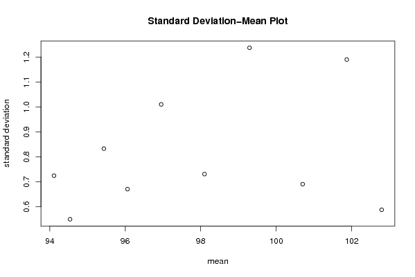
| Title produced by software | Standard Deviation-Mean Plot | ||||||||||||||||||||||||||||||||||||||||||||||||||||||||||||||||||||||||||||||||||||||||||||||||||||||||||||||||||||||||||||||||||||||||||||||||||||||||||||||||||||||||
| Date of computation | Sat, 06 Dec 2008 04:49:39 -0700 | ||||||||||||||||||||||||||||||||||||||||||||||||||||||||||||||||||||||||||||||||||||||||||||||||||||||||||||||||||||||||||||||||||||||||||||||||||||||||||||||||||||||||
| Cite this page as follows | Statistical Computations at FreeStatistics.org, Office for Research Development and Education, URL https://freestatistics.org/blog/index.php?v=date/2008/Dec/06/t1228564255gjc04aa6e7sjke4.htm/, Retrieved Sun, 19 May 2024 11:09:30 +0000 | ||||||||||||||||||||||||||||||||||||||||||||||||||||||||||||||||||||||||||||||||||||||||||||||||||||||||||||||||||||||||||||||||||||||||||||||||||||||||||||||||||||||||
| Statistical Computations at FreeStatistics.org, Office for Research Development and Education, URL https://freestatistics.org/blog/index.php?pk=29521, Retrieved Sun, 19 May 2024 11:09:30 +0000 | |||||||||||||||||||||||||||||||||||||||||||||||||||||||||||||||||||||||||||||||||||||||||||||||||||||||||||||||||||||||||||||||||||||||||||||||||||||||||||||||||||||||||
| QR Codes: | |||||||||||||||||||||||||||||||||||||||||||||||||||||||||||||||||||||||||||||||||||||||||||||||||||||||||||||||||||||||||||||||||||||||||||||||||||||||||||||||||||||||||
|
| |||||||||||||||||||||||||||||||||||||||||||||||||||||||||||||||||||||||||||||||||||||||||||||||||||||||||||||||||||||||||||||||||||||||||||||||||||||||||||||||||||||||||
| Original text written by user: | Seizonaal op 6 gezet in plaats van 12. | ||||||||||||||||||||||||||||||||||||||||||||||||||||||||||||||||||||||||||||||||||||||||||||||||||||||||||||||||||||||||||||||||||||||||||||||||||||||||||||||||||||||||
| IsPrivate? | No (this computation is public) | ||||||||||||||||||||||||||||||||||||||||||||||||||||||||||||||||||||||||||||||||||||||||||||||||||||||||||||||||||||||||||||||||||||||||||||||||||||||||||||||||||||||||
| User-defined keywords | |||||||||||||||||||||||||||||||||||||||||||||||||||||||||||||||||||||||||||||||||||||||||||||||||||||||||||||||||||||||||||||||||||||||||||||||||||||||||||||||||||||||||
| Estimated Impact | 289 | ||||||||||||||||||||||||||||||||||||||||||||||||||||||||||||||||||||||||||||||||||||||||||||||||||||||||||||||||||||||||||||||||||||||||||||||||||||||||||||||||||||||||
Tree of Dependent Computations | |||||||||||||||||||||||||||||||||||||||||||||||||||||||||||||||||||||||||||||||||||||||||||||||||||||||||||||||||||||||||||||||||||||||||||||||||||||||||||||||||||||||||
| Family? (F = Feedback message, R = changed R code, M = changed R Module, P = changed Parameters, D = changed Data) | |||||||||||||||||||||||||||||||||||||||||||||||||||||||||||||||||||||||||||||||||||||||||||||||||||||||||||||||||||||||||||||||||||||||||||||||||||||||||||||||||||||||||
| - [Univariate Data Series] [Run sequence plot...] [2008-12-02 22:19:27] [ed2ba3b6182103c15c0ab511ae4e6284] - RMPD [Standard Deviation-Mean Plot] [SD mean plot] [2008-12-06 11:49:39] [a8228479d4547a92e2d3f176a5299609] [Current] F RM [Variance Reduction Matrix] [variance reduction] [2008-12-06 12:44:59] [ed2ba3b6182103c15c0ab511ae4e6284] F D [Variance Reduction Matrix] [VRM Vlaanderen] [2008-12-08 18:29:56] [077ffec662d24c06be4c491541a44245] - RMPD [(Partial) Autocorrelation Function] [ACF] [2008-12-08 18:32:31] [077ffec662d24c06be4c491541a44245] - P [(Partial) Autocorrelation Function] [ACF] [2008-12-08 18:34:40] [077ffec662d24c06be4c491541a44245] - P [(Partial) Autocorrelation Function] [ACF] [2008-12-08 18:36:48] [077ffec662d24c06be4c491541a44245] - P [Variance Reduction Matrix] [variance reduction] [2008-12-08 19:33:22] [4ad596f10399a71ad29b7d76e6ab90ac] - [Variance Reduction Matrix] [variance reduction] [2008-12-09 00:17:49] [4ddbf81f78ea7c738951638c7e93f6ee] - [Variance Reduction Matrix] [] [2008-12-09 00:23:30] [29747f79f5beb5b2516e1271770ecb47] - RMP [(Partial) Autocorrelation Function] [ACF d=o en D=0] [2008-12-06 12:48:15] [ed2ba3b6182103c15c0ab511ae4e6284] - P [(Partial) Autocorrelation Function] [ACF d=0 en D=0 la...] [2008-12-07 15:39:10] [ed2ba3b6182103c15c0ab511ae4e6284] - P [(Partial) Autocorrelation Function] [acf ] [2008-12-08 11:41:37] [ed2ba3b6182103c15c0ab511ae4e6284] F P [(Partial) Autocorrelation Function] [acf] [2008-12-08 19:38:35] [4ad596f10399a71ad29b7d76e6ab90ac] F [(Partial) Autocorrelation Function] [] [2008-12-08 21:14:50] [28075c6928548bea087cb2be962cfe7e] - [(Partial) Autocorrelation Function] [ACF] [2008-12-09 00:20:22] [4ddbf81f78ea7c738951638c7e93f6ee] - [(Partial) Autocorrelation Function] [] [2008-12-09 00:24:15] [29747f79f5beb5b2516e1271770ecb47] - RMP [(Partial) Autocorrelation Function] [ACF d=1 en D=0] [2008-12-06 12:51:22] [ed2ba3b6182103c15c0ab511ae4e6284] - P [(Partial) Autocorrelation Function] [acf d=1] [2008-12-08 11:43:53] [74be16979710d4c4e7c6647856088456] - P [(Partial) Autocorrelation Function] [acf d=1] [2008-12-08 11:43:53] [ed2ba3b6182103c15c0ab511ae4e6284] - [(Partial) Autocorrelation Function] [acf d=1] [2008-12-08 19:45:09] [4ad596f10399a71ad29b7d76e6ab90ac] - [(Partial) Autocorrelation Function] [] [2008-12-08 21:16:19] [28075c6928548bea087cb2be962cfe7e] - [(Partial) Autocorrelation Function] [ACF d=1] [2008-12-09 00:23:10] [4ddbf81f78ea7c738951638c7e93f6ee] - [(Partial) Autocorrelation Function] [] [2008-12-09 00:25:46] [29747f79f5beb5b2516e1271770ecb47] - RMP [(Partial) Autocorrelation Function] [ACF d=1 en D=1] [2008-12-06 12:54:17] [ed2ba3b6182103c15c0ab511ae4e6284] - RMP [Spectral Analysis] [spectrum ] [2008-12-06 13:17:20] [ed2ba3b6182103c15c0ab511ae4e6284] F P [Spectral Analysis] [spectrale analyse] [2008-12-08 11:48:47] [ed2ba3b6182103c15c0ab511ae4e6284] - [Spectral Analysis] [Spectrum] [2008-12-08 19:51:12] [4ad596f10399a71ad29b7d76e6ab90ac] - [Spectral Analysis] [] [2008-12-08 21:24:23] [28075c6928548bea087cb2be962cfe7e] - [Spectral Analysis] [spectrale analyse] [2008-12-09 00:26:01] [4ddbf81f78ea7c738951638c7e93f6ee] - [Spectral Analysis] [spectrale analyse] [2008-12-09 00:28:17] [4ddbf81f78ea7c738951638c7e93f6ee] - [Spectral Analysis] [] [2008-12-09 00:31:58] [29747f79f5beb5b2516e1271770ecb47] - [Spectral Analysis] [] [2008-12-09 00:33:16] [29747f79f5beb5b2516e1271770ecb47] - PD [Spectral Analysis] [Q9 laatste taak p...] [2008-12-08 18:39:46] [077ffec662d24c06be4c491541a44245] F RMP [(Partial) Autocorrelation Function] [ACF d=1 en D=1 la...] [2008-12-06 13:30:27] [ed2ba3b6182103c15c0ab511ae4e6284] - RM [ARIMA Backward Selection] [ARIMA model met q...] [2008-12-06 17:04:18] [4242609301e759e844b9196c1994e4ef] - P [ARIMA Backward Selection] [ARima backward se...] [2008-12-08 11:53:47] [ed2ba3b6182103c15c0ab511ae4e6284] - P [ARIMA Backward Selection] [MA controle] [2008-12-08 11:58:59] [ed2ba3b6182103c15c0ab511ae4e6284] F [ARIMA Backward Selection] [ARIMA] [2008-12-08 20:02:58] [4ad596f10399a71ad29b7d76e6ab90ac] - RMP [ARIMA Forecasting] [ARIMA forecast HI...] [2008-12-13 14:12:52] [ed2ba3b6182103c15c0ab511ae4e6284] - [ARIMA Backward Selection] [] [2008-12-08 21:34:29] [28075c6928548bea087cb2be962cfe7e] - P [ARIMA Backward Selection] [] [2008-12-09 00:38:49] [29747f79f5beb5b2516e1271770ecb47] - [ARIMA Backward Selection] [ARIMA] [2008-12-08 20:00:39] [4ad596f10399a71ad29b7d76e6ab90ac] F [ARIMA Backward Selection] [] [2008-12-08 21:33:18] [28075c6928548bea087cb2be962cfe7e] - [ARIMA Backward Selection] [Arima backward se...] [2008-12-09 00:33:34] [4ddbf81f78ea7c738951638c7e93f6ee] - P [ARIMA Backward Selection] [] [2008-12-09 00:36:36] [29747f79f5beb5b2516e1271770ecb47] - [ARIMA Backward Selection] [Arima backward se...] [2008-12-09 00:33:34] [4ddbf81f78ea7c738951638c7e93f6ee] F RMP [ARIMA Forecasting] [ARIMA forecasting] [2008-12-09 20:21:38] [ed2ba3b6182103c15c0ab511ae4e6284] F [ARIMA Forecasting] [Arima forecasting...] [2008-12-15 09:55:01] [4ad596f10399a71ad29b7d76e6ab90ac] F [ARIMA Forecasting] [ARIMA forecasting] [2008-12-15 09:56:32] [7506b5e9e41ec66c6657f4234f97306e] [Truncated] | |||||||||||||||||||||||||||||||||||||||||||||||||||||||||||||||||||||||||||||||||||||||||||||||||||||||||||||||||||||||||||||||||||||||||||||||||||||||||||||||||||||||||
| Feedback Forum | |||||||||||||||||||||||||||||||||||||||||||||||||||||||||||||||||||||||||||||||||||||||||||||||||||||||||||||||||||||||||||||||||||||||||||||||||||||||||||||||||||||||||
Post a new message | |||||||||||||||||||||||||||||||||||||||||||||||||||||||||||||||||||||||||||||||||||||||||||||||||||||||||||||||||||||||||||||||||||||||||||||||||||||||||||||||||||||||||
Dataset | |||||||||||||||||||||||||||||||||||||||||||||||||||||||||||||||||||||||||||||||||||||||||||||||||||||||||||||||||||||||||||||||||||||||||||||||||||||||||||||||||||||||||
| Dataseries X: | |||||||||||||||||||||||||||||||||||||||||||||||||||||||||||||||||||||||||||||||||||||||||||||||||||||||||||||||||||||||||||||||||||||||||||||||||||||||||||||||||||||||||
92.66 94.2 94.37 94.45 94.62 94.37 93.43 94.79 94.88 94.79 94.62 94.71 93.77 95.73 95.99 95.82 95.47 95.82 94.71 96.33 96.5 96.16 96.33 96.33 95.05 96.84 96.92 97.44 97.78 97.69 96.67 98.29 98.2 98.71 98.54 98.2 96.92 99.06 99.65 99.82 99.99 100.33 99.31 101.1 101.1 100.93 100.85 100.93 99.6 101.88 101.81 102.38 102.74 102.82 101.72 103.47 102.98 102.68 102.9 103.03 101.29 | |||||||||||||||||||||||||||||||||||||||||||||||||||||||||||||||||||||||||||||||||||||||||||||||||||||||||||||||||||||||||||||||||||||||||||||||||||||||||||||||||||||||||
Tables (Output of Computation) | |||||||||||||||||||||||||||||||||||||||||||||||||||||||||||||||||||||||||||||||||||||||||||||||||||||||||||||||||||||||||||||||||||||||||||||||||||||||||||||||||||||||||
| |||||||||||||||||||||||||||||||||||||||||||||||||||||||||||||||||||||||||||||||||||||||||||||||||||||||||||||||||||||||||||||||||||||||||||||||||||||||||||||||||||||||||
Figures (Output of Computation) | |||||||||||||||||||||||||||||||||||||||||||||||||||||||||||||||||||||||||||||||||||||||||||||||||||||||||||||||||||||||||||||||||||||||||||||||||||||||||||||||||||||||||
Input Parameters & R Code | |||||||||||||||||||||||||||||||||||||||||||||||||||||||||||||||||||||||||||||||||||||||||||||||||||||||||||||||||||||||||||||||||||||||||||||||||||||||||||||||||||||||||
| Parameters (Session): | |||||||||||||||||||||||||||||||||||||||||||||||||||||||||||||||||||||||||||||||||||||||||||||||||||||||||||||||||||||||||||||||||||||||||||||||||||||||||||||||||||||||||
| par1 = 6 ; | |||||||||||||||||||||||||||||||||||||||||||||||||||||||||||||||||||||||||||||||||||||||||||||||||||||||||||||||||||||||||||||||||||||||||||||||||||||||||||||||||||||||||
| Parameters (R input): | |||||||||||||||||||||||||||||||||||||||||||||||||||||||||||||||||||||||||||||||||||||||||||||||||||||||||||||||||||||||||||||||||||||||||||||||||||||||||||||||||||||||||
| par1 = 6 ; | |||||||||||||||||||||||||||||||||||||||||||||||||||||||||||||||||||||||||||||||||||||||||||||||||||||||||||||||||||||||||||||||||||||||||||||||||||||||||||||||||||||||||
| R code (references can be found in the software module): | |||||||||||||||||||||||||||||||||||||||||||||||||||||||||||||||||||||||||||||||||||||||||||||||||||||||||||||||||||||||||||||||||||||||||||||||||||||||||||||||||||||||||
par1 <- as.numeric(par1) | |||||||||||||||||||||||||||||||||||||||||||||||||||||||||||||||||||||||||||||||||||||||||||||||||||||||||||||||||||||||||||||||||||||||||||||||||||||||||||||||||||||||||