Repository of Reproducible Computations

Free Statistics

of Irreproducible Research!

Author's title

Author

*The author of this computation has been verified*

R Software Module

rwasp_autocorrelation.wasp

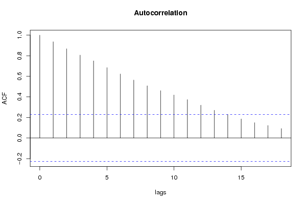
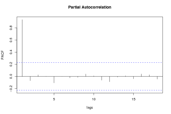
Title produced by software

(Partial) Autocorrelation Function

Date of computation

Sat, 06 Dec 2008 03:52:06 -0700

Cite this page as follows

Statistical Computations at FreeStatistics.org, Office for Research Development and Education, URL https://freestatistics.org/blog/index.php?v=date/2008/Dec/06/t1228560916433rz9u4vrufqa5.htm/, Retrieved Sun, 19 May 2024 08:52:31 +0000

Statistical Computations at FreeStatistics.org, Office for Research Development and Education, URL https://freestatistics.org/blog/index.php?pk=29493, Retrieved Sun, 19 May 2024 08:52:31 +0000

QR Codes:

Paste this QR Code to cite your computation.

Original text written by user:

IsPrivate?

No (this computation is public)

User-defined keywords

Estimated Impact

198

Family? (F = Feedback message, R = changed R code, M = changed R Module, P = changed Parameters, D = changed Data)

-     [Univariate Data Series] [data set] [2008-12-01 19:54:57] [b98453cac15ba1066b407e146608df68]
F RMP   [Standard Deviation-Mean Plot] [sdm ] [2008-12-05 13:33:27] [de72ca3f4fcfd0997c84e1ac92aea119]
F RM D    [Variance Reduction Matrix] [Q2 eigen tijdreeks] [2008-12-06 10:45:14] [de72ca3f4fcfd0997c84e1ac92aea119]
F RMP         [(Partial) Autocorrelation Function] [Q2 eigen tijdreeks] [2008-12-06 10:52:06] [56fd94b954e08a6655cb7790b21ee404] [Current]
F RMP           [Spectral Analysis] [Q2 eigen tijdreeks] [2008-12-06 10:56:27] [de72ca3f4fcfd0997c84e1ac92aea119] 
-   P             [Spectral Analysis] [Q3 Eigen tijdreeks] [2008-12-06 11:07:10] [de72ca3f4fcfd0997c84e1ac92aea119] 
-   P               [Spectral Analysis] [Q3 Eigen tijdreeks] [2008-12-06 13:01:00] [de72ca3f4fcfd0997c84e1ac92aea119] 
-   P           [(Partial) Autocorrelation Function] [Q3 Eigen tijdreeks] [2008-12-06 13:06:08] [de72ca3f4fcfd0997c84e1ac92aea119] 
-   P             [(Partial) Autocorrelation Function] [Q3 Eigen tijdreeks] [2008-12-06 13:14:50] [de72ca3f4fcfd0997c84e1ac92aea119] 

Feedback Forum

2008-12-14 14:20:07 [Hannes Van Hoof] [reply] 
De ACF bevestigt wat we gevonden hebben in de VRM Er is enkel een LT trend aanwezig en moeten dus enkel niet seizoenaal differentiëren. 
Seizoenaliteit zien we niet op deze ACF

Post a new message

Dataseries X:

Download CSV

Histogram

Boxplots

Summary of computational transaction
Raw Input	view raw input (R code)
Raw Output	view raw output of R engine
Computing time	1 seconds
R Server	'Gwilym Jenkins' @ 72.249.127.135

\begin{tabular}{lllllllll}
\hline
Summary of computational transaction \tabularnewline
Raw Input & view raw input (R code)  \tabularnewline
Raw Output & view raw output of R engine  \tabularnewline
Computing time & 1 seconds \tabularnewline
R Server & 'Gwilym Jenkins' @ 72.249.127.135 \tabularnewline
\hline
\end{tabular}
%Source: https://freestatistics.org/blog/index.php?pk=29493&T=0

[TABLE]
[ROW][C]Summary of computational transaction[/C][/ROW]
[ROW][C]Raw Input[/C][C]view raw input (R code) [/C][/ROW]
[ROW][C]Raw Output[/C][C]view raw output of R engine [/C][/ROW]
[ROW][C]Computing time[/C][C]1 seconds[/C][/ROW]
[ROW][C]R Server[/C][C]'Gwilym Jenkins' @ 72.249.127.135[/C][/ROW]
[/TABLE]
Source: https://freestatistics.org/blog/index.php?pk=29493&T=0

Globally Unique Identifier (entire table): ba.freestatistics.org/blog/index.php?pk=29493&T=0

As an alternative you can also use a QR Code:

The GUIDs for individual cells are displayed in the table below:

Summary of computational transaction
Raw Input	view raw input (R code)
Raw Output	view raw output of R engine
Computing time	1 seconds
R Server	'Gwilym Jenkins' @ 72.249.127.135

Autocorrelation Function
Time lag k	ACF(k)	T-STAT	P-value
1	0.935964	8.0515	0
2	0.867251	7.4604	0
3	0.806251	6.9356	0
4	0.750187	6.4534	0
5	0.684807	5.8909	0
6	0.622898	5.3584	0
7	0.56388	4.8507	3e-06
8	0.507939	4.3695	2e-05
9	0.460477	3.9612	8.5e-05
10	0.419114	3.6054	0.000281
11	0.373458	3.2126	0.000974
12	0.319883	2.7517	0.003725
13	0.270346	2.3256	0.011391
14	0.228515	1.9658	0.026539
15	0.185655	1.5971	0.057257
16	0.149818	1.2888	0.100744
17	0.121892	1.0486	0.148899
18	0.092648	0.797	0.214004

\begin{tabular}{lllllllll}
\hline
Autocorrelation Function \tabularnewline
Time lag k & ACF(k) & T-STAT & P-value \tabularnewline
1 & 0.935964 & 8.0515 & 0 \tabularnewline
2 & 0.867251 & 7.4604 & 0 \tabularnewline
3 & 0.806251 & 6.9356 & 0 \tabularnewline
4 & 0.750187 & 6.4534 & 0 \tabularnewline
5 & 0.684807 & 5.8909 & 0 \tabularnewline
6 & 0.622898 & 5.3584 & 0 \tabularnewline
7 & 0.56388 & 4.8507 & 3e-06 \tabularnewline
8 & 0.507939 & 4.3695 & 2e-05 \tabularnewline
9 & 0.460477 & 3.9612 & 8.5e-05 \tabularnewline
10 & 0.419114 & 3.6054 & 0.000281 \tabularnewline
11 & 0.373458 & 3.2126 & 0.000974 \tabularnewline
12 & 0.319883 & 2.7517 & 0.003725 \tabularnewline
13 & 0.270346 & 2.3256 & 0.011391 \tabularnewline
14 & 0.228515 & 1.9658 & 0.026539 \tabularnewline
15 & 0.185655 & 1.5971 & 0.057257 \tabularnewline
16 & 0.149818 & 1.2888 & 0.100744 \tabularnewline
17 & 0.121892 & 1.0486 & 0.148899 \tabularnewline
18 & 0.092648 & 0.797 & 0.214004 \tabularnewline
\hline
\end{tabular}
%Source: https://freestatistics.org/blog/index.php?pk=29493&T=1

[TABLE]
[ROW][C]Autocorrelation Function[/C][/ROW]
[ROW][C]Time lag k[/C][C]ACF(k)[/C][C]T-STAT[/C][C]P-value[/C][/ROW]
[ROW][C]1[/C][C]0.935964[/C][C]8.0515[/C][C]0[/C][/ROW]
[ROW][C]2[/C][C]0.867251[/C][C]7.4604[/C][C]0[/C][/ROW]
[ROW][C]3[/C][C]0.806251[/C][C]6.9356[/C][C]0[/C][/ROW]
[ROW][C]4[/C][C]0.750187[/C][C]6.4534[/C][C]0[/C][/ROW]
[ROW][C]5[/C][C]0.684807[/C][C]5.8909[/C][C]0[/C][/ROW]
[ROW][C]6[/C][C]0.622898[/C][C]5.3584[/C][C]0[/C][/ROW]
[ROW][C]7[/C][C]0.56388[/C][C]4.8507[/C][C]3e-06[/C][/ROW]
[ROW][C]8[/C][C]0.507939[/C][C]4.3695[/C][C]2e-05[/C][/ROW]
[ROW][C]9[/C][C]0.460477[/C][C]3.9612[/C][C]8.5e-05[/C][/ROW]
[ROW][C]10[/C][C]0.419114[/C][C]3.6054[/C][C]0.000281[/C][/ROW]
[ROW][C]11[/C][C]0.373458[/C][C]3.2126[/C][C]0.000974[/C][/ROW]
[ROW][C]12[/C][C]0.319883[/C][C]2.7517[/C][C]0.003725[/C][/ROW]
[ROW][C]13[/C][C]0.270346[/C][C]2.3256[/C][C]0.011391[/C][/ROW]
[ROW][C]14[/C][C]0.228515[/C][C]1.9658[/C][C]0.026539[/C][/ROW]
[ROW][C]15[/C][C]0.185655[/C][C]1.5971[/C][C]0.057257[/C][/ROW]
[ROW][C]16[/C][C]0.149818[/C][C]1.2888[/C][C]0.100744[/C][/ROW]
[ROW][C]17[/C][C]0.121892[/C][C]1.0486[/C][C]0.148899[/C][/ROW]
[ROW][C]18[/C][C]0.092648[/C][C]0.797[/C][C]0.214004[/C][/ROW]
[/TABLE]
Source: https://freestatistics.org/blog/index.php?pk=29493&T=1

Globally Unique Identifier (entire table): ba.freestatistics.org/blog/index.php?pk=29493&T=1

As an alternative you can also use a QR Code:

The GUIDs for individual cells are displayed in the table below:

Autocorrelation Function
Time lag k	ACF(k)	T-STAT	P-value
1	0.935964	8.0515	0
2	0.867251	7.4604	0
3	0.806251	6.9356	0
4	0.750187	6.4534	0
5	0.684807	5.8909	0
6	0.622898	5.3584	0
7	0.56388	4.8507	3e-06
8	0.507939	4.3695	2e-05
9	0.460477	3.9612	8.5e-05
10	0.419114	3.6054	0.000281
11	0.373458	3.2126	0.000974
12	0.319883	2.7517	0.003725
13	0.270346	2.3256	0.011391
14	0.228515	1.9658	0.026539
15	0.185655	1.5971	0.057257
16	0.149818	1.2888	0.100744
17	0.121892	1.0486	0.148899
18	0.092648	0.797	0.214004

Partial Autocorrelation Function
Time lag k	PACF(k)	T-STAT	P-value
1	0.935964	8.0515	0
2	-0.070802	-0.6091	0.272175
3	0.027014	0.2324	0.40844
4	0.00157	0.0135	0.49463
5	-0.107086	-0.9212	0.179973
6	-0.000186	-0.0016	0.499363
7	-0.023967	-0.2062	0.418611
8	-0.016244	-0.1397	0.444624
9	0.040252	0.3463	0.365063
10	0.009805	0.0843	0.466503
11	-0.062147	-0.5346	0.29726
12	-0.088526	-0.7615	0.224381
13	-0.01139	-0.098	0.461106
14	0.011281	0.097	0.461477
15	-0.039942	-0.3436	0.366063
16	0.040858	0.3515	0.363117
17	0.027561	0.2371	0.406622
18	-0.044526	-0.383	0.3514

\begin{tabular}{lllllllll}
\hline
Partial Autocorrelation Function \tabularnewline
Time lag k & PACF(k) & T-STAT & P-value \tabularnewline
1 & 0.935964 & 8.0515 & 0 \tabularnewline
2 & -0.070802 & -0.6091 & 0.272175 \tabularnewline
3 & 0.027014 & 0.2324 & 0.40844 \tabularnewline
4 & 0.00157 & 0.0135 & 0.49463 \tabularnewline
5 & -0.107086 & -0.9212 & 0.179973 \tabularnewline
6 & -0.000186 & -0.0016 & 0.499363 \tabularnewline
7 & -0.023967 & -0.2062 & 0.418611 \tabularnewline
8 & -0.016244 & -0.1397 & 0.444624 \tabularnewline
9 & 0.040252 & 0.3463 & 0.365063 \tabularnewline
10 & 0.009805 & 0.0843 & 0.466503 \tabularnewline
11 & -0.062147 & -0.5346 & 0.29726 \tabularnewline
12 & -0.088526 & -0.7615 & 0.224381 \tabularnewline
13 & -0.01139 & -0.098 & 0.461106 \tabularnewline
14 & 0.011281 & 0.097 & 0.461477 \tabularnewline
15 & -0.039942 & -0.3436 & 0.366063 \tabularnewline
16 & 0.040858 & 0.3515 & 0.363117 \tabularnewline
17 & 0.027561 & 0.2371 & 0.406622 \tabularnewline
18 & -0.044526 & -0.383 & 0.3514 \tabularnewline
\hline
\end{tabular}
%Source: https://freestatistics.org/blog/index.php?pk=29493&T=2

[TABLE]
[ROW][C]Partial Autocorrelation Function[/C][/ROW]
[ROW][C]Time lag k[/C][C]PACF(k)[/C][C]T-STAT[/C][C]P-value[/C][/ROW]
[ROW][C]1[/C][C]0.935964[/C][C]8.0515[/C][C]0[/C][/ROW]
[ROW][C]2[/C][C]-0.070802[/C][C]-0.6091[/C][C]0.272175[/C][/ROW]
[ROW][C]3[/C][C]0.027014[/C][C]0.2324[/C][C]0.40844[/C][/ROW]
[ROW][C]4[/C][C]0.00157[/C][C]0.0135[/C][C]0.49463[/C][/ROW]
[ROW][C]5[/C][C]-0.107086[/C][C]-0.9212[/C][C]0.179973[/C][/ROW]
[ROW][C]6[/C][C]-0.000186[/C][C]-0.0016[/C][C]0.499363[/C][/ROW]
[ROW][C]7[/C][C]-0.023967[/C][C]-0.2062[/C][C]0.418611[/C][/ROW]
[ROW][C]8[/C][C]-0.016244[/C][C]-0.1397[/C][C]0.444624[/C][/ROW]
[ROW][C]9[/C][C]0.040252[/C][C]0.3463[/C][C]0.365063[/C][/ROW]
[ROW][C]10[/C][C]0.009805[/C][C]0.0843[/C][C]0.466503[/C][/ROW]
[ROW][C]11[/C][C]-0.062147[/C][C]-0.5346[/C][C]0.29726[/C][/ROW]
[ROW][C]12[/C][C]-0.088526[/C][C]-0.7615[/C][C]0.224381[/C][/ROW]
[ROW][C]13[/C][C]-0.01139[/C][C]-0.098[/C][C]0.461106[/C][/ROW]
[ROW][C]14[/C][C]0.011281[/C][C]0.097[/C][C]0.461477[/C][/ROW]
[ROW][C]15[/C][C]-0.039942[/C][C]-0.3436[/C][C]0.366063[/C][/ROW]
[ROW][C]16[/C][C]0.040858[/C][C]0.3515[/C][C]0.363117[/C][/ROW]
[ROW][C]17[/C][C]0.027561[/C][C]0.2371[/C][C]0.406622[/C][/ROW]
[ROW][C]18[/C][C]-0.044526[/C][C]-0.383[/C][C]0.3514[/C][/ROW]
[/TABLE]
Source: https://freestatistics.org/blog/index.php?pk=29493&T=2

Globally Unique Identifier (entire table): ba.freestatistics.org/blog/index.php?pk=29493&T=2

As an alternative you can also use a QR Code:

The GUIDs for individual cells are displayed in the table below:

Partial Autocorrelation Function
Time lag k	PACF(k)	T-STAT	P-value
1	0.935964	8.0515	0
2	-0.070802	-0.6091	0.272175
3	0.027014	0.2324	0.40844
4	0.00157	0.0135	0.49463
5	-0.107086	-0.9212	0.179973
6	-0.000186	-0.0016	0.499363
7	-0.023967	-0.2062	0.418611
8	-0.016244	-0.1397	0.444624
9	0.040252	0.3463	0.365063
10	0.009805	0.0843	0.466503
11	-0.062147	-0.5346	0.29726
12	-0.088526	-0.7615	0.224381
13	-0.01139	-0.098	0.461106
14	0.011281	0.097	0.461477
15	-0.039942	-0.3436	0.366063
16	0.040858	0.3515	0.363117
17	0.027561	0.2371	0.406622
18	-0.044526	-0.383	0.3514

Figure 1

PNG link

Postscript link

PDF link

Figure 2

PNG link

Postscript link

PDF link

Parameters (Session):

par1 = Default ; par2 = 1 ; par3 = 0 ; par4 = 0 ; par5 = 12 ;

Parameters (R input):

par1 = Default ; par2 = 1 ; par3 = 0 ; par4 = 0 ; par5 = 12 ;

R code (references can be found in the software module):

if (par1 == 'Default') {
par1 = 10*log10(length(x))
} else {
par1 <- as.numeric(par1)
}
par2 <- as.numeric(par2)
par3 <- as.numeric(par3)
par4 <- as.numeric(par4)
par5 <- as.numeric(par5)
if (par2 == 0) {
x <- log(x)
} else {
x <- (x ^ par2 - 1) / par2
}
if (par3 > 0) x <- diff(x,lag=1,difference=par3)
if (par4 > 0) x <- diff(x,lag=par5,difference=par4)
bitmap(file='pic1.png')
racf <- acf(x,par1,main='Autocorrelation',xlab='lags',ylab='ACF')
dev.off()
bitmap(file='pic2.png')
rpacf <- pacf(x,par1,main='Partial Autocorrelation',xlab='lags',ylab='PACF')
dev.off()
(myacf <- c(racf$acf))
(mypacf <- c(rpacf$acf))
lengthx <- length(x)
sqrtn <- sqrt(lengthx)
load(file='createtable')
a<-table.start()
a<-table.row.start(a)
a<-table.element(a,'Autocorrelation Function',4,TRUE)
a<-table.row.end(a)
a<-table.row.start(a)
a<-table.element(a,'Time lag k',header=TRUE)
a<-table.element(a,hyperlink('basics.htm','ACF(k)','click here for more information about the Autocorrelation Function'),header=TRUE)
a<-table.element(a,'T-STAT',header=TRUE)
a<-table.element(a,'P-value',header=TRUE)
a<-table.row.end(a)
for (i in 2:(par1+1)) {
a<-table.row.start(a)
a<-table.element(a,i-1,header=TRUE)
a<-table.element(a,round(myacf[i],6))
mytstat <- myacf[i]*sqrtn
a<-table.element(a,round(mytstat,4))
a<-table.element(a,round(1-pt(abs(mytstat),lengthx),6))
a<-table.row.end(a)
}
a<-table.end(a)
table.save(a,file='mytable.tab')
a<-table.start()
a<-table.row.start(a)
a<-table.element(a,'Partial Autocorrelation Function',4,TRUE)
a<-table.row.end(a)
a<-table.row.start(a)
a<-table.element(a,'Time lag k',header=TRUE)
a<-table.element(a,hyperlink('basics.htm','PACF(k)','click here for more information about the Partial Autocorrelation Function'),header=TRUE)
a<-table.element(a,'T-STAT',header=TRUE)
a<-table.element(a,'P-value',header=TRUE)
a<-table.row.end(a)
for (i in 1:par1) {
a<-table.row.start(a)
a<-table.element(a,i,header=TRUE)
a<-table.element(a,round(mypacf[i],6))
mytstat <- mypacf[i]*sqrtn
a<-table.element(a,round(mytstat,4))
a<-table.element(a,round(1-pt(abs(mytstat),lengthx),6))
a<-table.row.end(a)
}
a<-table.end(a)
table.save(a,file='mytable1.tab')

Free Statistics

Description of Statistical Computation

Tree of Dependent Computations

Dataset

Tables (Output of Computation)

Figures (Output of Computation)

Input Parameters & R Code