Repository of Reproducible Computations

Free Statistics

of Irreproducible Research!

Author's title

Author

*The author of this computation has been verified*

R Software Module

rwasp_autocorrelation.wasp

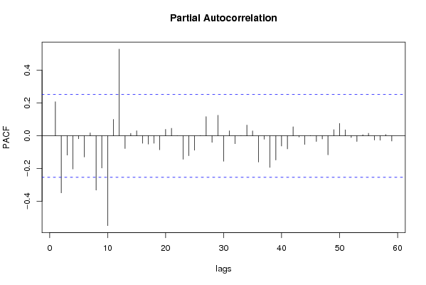
Title produced by software

(Partial) Autocorrelation Function

Date of computation

Wed, 03 Dec 2008 09:37:45 -0700

Cite this page as follows

Statistical Computations at FreeStatistics.org, Office for Research Development and Education, URL https://freestatistics.org/blog/index.php?v=date/2008/Dec/03/t1228322332j1k240yllgok6ow.htm/, Retrieved Sun, 19 May 2024 04:11:52 +0000

Statistical Computations at FreeStatistics.org, Office for Research Development and Education, URL https://freestatistics.org/blog/index.php?pk=28777, Retrieved Sun, 19 May 2024 04:11:52 +0000

QR Codes:

Paste this QR Code to cite your computation.

Original text written by user:

IsPrivate?

No (this computation is public)

User-defined keywords

Estimated Impact

214

Family? (F = Feedback message, R = changed R code, M = changed R Module, P = changed Parameters, D = changed Data)

-     [Univariate Data Series] [data set] [2008-12-01 19:54:57] [b98453cac15ba1066b407e146608df68]
- RMPD  [(Partial) Autocorrelation Function] [taak 8 werklozen ...] [2008-12-03 16:32:44] [e1a46c1dcfccb0cb690f79a1a409b517]
-   P       [(Partial) Autocorrelation Function] [taak 8 werklozen ...] [2008-12-03 16:37:45] [bda7fba231d49184c6a1b627868bbb81] [Current]
-   P         [(Partial) Autocorrelation Function] [taak 8 werklozen ...] [2008-12-03 16:39:57] [e1a46c1dcfccb0cb690f79a1a409b517] 
-   P         [(Partial) Autocorrelation Function] [taak 8 werklozen ...] [2008-12-03 16:44:22] [e1a46c1dcfccb0cb690f79a1a409b517] 
- RMP         [Spectral Analysis] [taak 8 werklozen ...] [2008-12-03 16:47:41] [e1a46c1dcfccb0cb690f79a1a409b517] 
-   P           [Spectral Analysis] [taak 8 werklozen ...] [2008-12-03 16:51:44] [e1a46c1dcfccb0cb690f79a1a409b517] 
-   P             [Spectral Analysis] [taak 8 werklozen ...] [2008-12-03 16:54:18] [e1a46c1dcfccb0cb690f79a1a409b517] 
- RMP               [Standard Deviation-Mean Plot] [taak 8 werklozen ...] [2008-12-03 16:58:07] [e1a46c1dcfccb0cb690f79a1a409b517] 
- RM                  [(Partial) Autocorrelation Function] [taak 8 werklozen ...] [2008-12-03 17:08:52] [e1a46c1dcfccb0cb690f79a1a409b517] 
-   P                   [(Partial) Autocorrelation Function] [taak 8 werklozen ...] [2008-12-05 11:44:45] [e1a46c1dcfccb0cb690f79a1a409b517] 
- RMP                     [ARIMA Backward Selection] [taak 8 werklozen ...] [2008-12-05 12:02:13] [e1a46c1dcfccb0cb690f79a1a409b517] 
-   P                       [ARIMA Backward Selection] [taak 8 werklozen ...] [2008-12-08 17:17:01] [e1a46c1dcfccb0cb690f79a1a409b517] 
- RMP                         [Univariate Data Series] [Time plot werkloo...] [2008-12-09 15:43:17] [e1a46c1dcfccb0cb690f79a1a409b517] 
-   P                     [(Partial) Autocorrelation Function] [Paper: Partial au...] [2008-12-13 09:24:08] [e1a46c1dcfccb0cb690f79a1a409b517] 

Feedback Forum

Post a new message

Dataseries X:

Download CSV

Histogram

Boxplots

Summary of computational transaction
Raw Input	view raw input (R code)
Raw Output	view raw output of R engine
Computing time	1 seconds
R Server	'George Udny Yule' @ 72.249.76.132

\begin{tabular}{lllllllll}
\hline
Summary of computational transaction \tabularnewline
Raw Input & view raw input (R code)  \tabularnewline
Raw Output & view raw output of R engine  \tabularnewline
Computing time & 1 seconds \tabularnewline
R Server & 'George Udny Yule' @ 72.249.76.132 \tabularnewline
\hline
\end{tabular}
%Source: https://freestatistics.org/blog/index.php?pk=28777&T=0

[TABLE]
[ROW][C]Summary of computational transaction[/C][/ROW]
[ROW][C]Raw Input[/C][C]view raw input (R code) [/C][/ROW]
[ROW][C]Raw Output[/C][C]view raw output of R engine [/C][/ROW]
[ROW][C]Computing time[/C][C]1 seconds[/C][/ROW]
[ROW][C]R Server[/C][C]'George Udny Yule' @ 72.249.76.132[/C][/ROW]
[/TABLE]
Source: https://freestatistics.org/blog/index.php?pk=28777&T=0

Globally Unique Identifier (entire table): ba.freestatistics.org/blog/index.php?pk=28777&T=0

As an alternative you can also use a QR Code:

The GUIDs for individual cells are displayed in the table below:

Summary of computational transaction
Raw Input	view raw input (R code)
Raw Output	view raw output of R engine
Computing time	1 seconds
R Server	'George Udny Yule' @ 72.249.76.132

Autocorrelation Function
Time lag k	ACF(k)	T-STAT	P-value
1	0.20774	1.6091	0.056417
2	-0.289975	-2.2461	0.014195
3	-0.252559	-1.9563	0.027544
4	-0.161321	-1.2496	0.108151
5	0.024375	0.1888	0.425442
6	0.03668	0.2841	0.388647
7	0.05838	0.4522	0.326373
8	-0.185596	-1.4376	0.077868
9	-0.238892	-1.8505	0.034587
10	-0.255327	-1.9778	0.026277
11	0.220482	1.7078	0.046418
12	0.778233	6.0282	0
13	0.161076	1.2477	0.108497
14	-0.253194	-1.9612	0.027249
15	-0.223245	-1.7292	0.044453
16	-0.125451	-0.9717	0.167541
17	-0.011971	-0.0927	0.463214
18	0.050097	0.388	0.349678
19	0.05487	0.425	0.336172
20	-0.151849	-1.1762	0.122078
21	-0.184405	-1.4284	0.079182
22	-0.197956	-1.5334	0.065221
23	0.165598	1.2827	0.102262
24	0.559906	4.337	2.8e-05
25	0.122328	0.9476	0.173579
26	-0.182345	-1.4124	0.081494
27	-0.115082	-0.8914	0.188132
28	-0.092937	-0.7199	0.237194
29	-0.007482	-0.058	0.476988
30	0.006916	0.0536	0.478727
31	0.037408	0.2898	0.386499
32	-0.094734	-0.7338	0.232961
33	-0.132377	-1.0254	0.154648
34	-0.114439	-0.8864	0.189459
35	0.099489	0.7706	0.221972
36	0.340841	2.6401	0.005273
37	0.053753	0.4164	0.339314
38	-0.126559	-0.9803	0.165432
39	-0.063813	-0.4943	0.311452
40	-0.041998	-0.3253	0.373038
41	-0.008649	-0.067	0.473405
42	-0.002325	-0.018	0.492845
43	0.034748	0.2692	0.394366
44	-0.055346	-0.4287	0.334836
45	-0.046084	-0.357	0.361184
46	-0.039541	-0.3063	0.380225
47	0.056078	0.4344	0.332785
48	0.145226	1.1249	0.132552
49	-0.002186	-0.0169	0.493274
50	-0.041358	-0.3204	0.374905
51	-0.009779	-0.0757	0.469937
52	0.002153	0.0167	0.493374
53	-0.002295	-0.0178	0.492938
54	0.009411	0.0729	0.471066
55	0.017479	0.1354	0.446379
56	-0.027524	-0.2132	0.415947
57	-0.022043	-0.1707	0.432499
58	0.010347	0.0801	0.468193
59	0.007025	0.0544	0.478392
60	NA	NA	NA

\begin{tabular}{lllllllll}
\hline
Autocorrelation Function \tabularnewline
Time lag k & ACF(k) & T-STAT & P-value \tabularnewline
1 & 0.20774 & 1.6091 & 0.056417 \tabularnewline
2 & -0.289975 & -2.2461 & 0.014195 \tabularnewline
3 & -0.252559 & -1.9563 & 0.027544 \tabularnewline
4 & -0.161321 & -1.2496 & 0.108151 \tabularnewline
5 & 0.024375 & 0.1888 & 0.425442 \tabularnewline
6 & 0.03668 & 0.2841 & 0.388647 \tabularnewline
7 & 0.05838 & 0.4522 & 0.326373 \tabularnewline
8 & -0.185596 & -1.4376 & 0.077868 \tabularnewline
9 & -0.238892 & -1.8505 & 0.034587 \tabularnewline
10 & -0.255327 & -1.9778 & 0.026277 \tabularnewline
11 & 0.220482 & 1.7078 & 0.046418 \tabularnewline
12 & 0.778233 & 6.0282 & 0 \tabularnewline
13 & 0.161076 & 1.2477 & 0.108497 \tabularnewline
14 & -0.253194 & -1.9612 & 0.027249 \tabularnewline
15 & -0.223245 & -1.7292 & 0.044453 \tabularnewline
16 & -0.125451 & -0.9717 & 0.167541 \tabularnewline
17 & -0.011971 & -0.0927 & 0.463214 \tabularnewline
18 & 0.050097 & 0.388 & 0.349678 \tabularnewline
19 & 0.05487 & 0.425 & 0.336172 \tabularnewline
20 & -0.151849 & -1.1762 & 0.122078 \tabularnewline
21 & -0.184405 & -1.4284 & 0.079182 \tabularnewline
22 & -0.197956 & -1.5334 & 0.065221 \tabularnewline
23 & 0.165598 & 1.2827 & 0.102262 \tabularnewline
24 & 0.559906 & 4.337 & 2.8e-05 \tabularnewline
25 & 0.122328 & 0.9476 & 0.173579 \tabularnewline
26 & -0.182345 & -1.4124 & 0.081494 \tabularnewline
27 & -0.115082 & -0.8914 & 0.188132 \tabularnewline
28 & -0.092937 & -0.7199 & 0.237194 \tabularnewline
29 & -0.007482 & -0.058 & 0.476988 \tabularnewline
30 & 0.006916 & 0.0536 & 0.478727 \tabularnewline
31 & 0.037408 & 0.2898 & 0.386499 \tabularnewline
32 & -0.094734 & -0.7338 & 0.232961 \tabularnewline
33 & -0.132377 & -1.0254 & 0.154648 \tabularnewline
34 & -0.114439 & -0.8864 & 0.189459 \tabularnewline
35 & 0.099489 & 0.7706 & 0.221972 \tabularnewline
36 & 0.340841 & 2.6401 & 0.005273 \tabularnewline
37 & 0.053753 & 0.4164 & 0.339314 \tabularnewline
38 & -0.126559 & -0.9803 & 0.165432 \tabularnewline
39 & -0.063813 & -0.4943 & 0.311452 \tabularnewline
40 & -0.041998 & -0.3253 & 0.373038 \tabularnewline
41 & -0.008649 & -0.067 & 0.473405 \tabularnewline
42 & -0.002325 & -0.018 & 0.492845 \tabularnewline
43 & 0.034748 & 0.2692 & 0.394366 \tabularnewline
44 & -0.055346 & -0.4287 & 0.334836 \tabularnewline
45 & -0.046084 & -0.357 & 0.361184 \tabularnewline
46 & -0.039541 & -0.3063 & 0.380225 \tabularnewline
47 & 0.056078 & 0.4344 & 0.332785 \tabularnewline
48 & 0.145226 & 1.1249 & 0.132552 \tabularnewline
49 & -0.002186 & -0.0169 & 0.493274 \tabularnewline
50 & -0.041358 & -0.3204 & 0.374905 \tabularnewline
51 & -0.009779 & -0.0757 & 0.469937 \tabularnewline
52 & 0.002153 & 0.0167 & 0.493374 \tabularnewline
53 & -0.002295 & -0.0178 & 0.492938 \tabularnewline
54 & 0.009411 & 0.0729 & 0.471066 \tabularnewline
55 & 0.017479 & 0.1354 & 0.446379 \tabularnewline
56 & -0.027524 & -0.2132 & 0.415947 \tabularnewline
57 & -0.022043 & -0.1707 & 0.432499 \tabularnewline
58 & 0.010347 & 0.0801 & 0.468193 \tabularnewline
59 & 0.007025 & 0.0544 & 0.478392 \tabularnewline
60 & NA & NA & NA \tabularnewline
\hline
\end{tabular}
%Source: https://freestatistics.org/blog/index.php?pk=28777&T=1

[TABLE]
[ROW][C]Autocorrelation Function[/C][/ROW]
[ROW][C]Time lag k[/C][C]ACF(k)[/C][C]T-STAT[/C][C]P-value[/C][/ROW]
[ROW][C]1[/C][C]0.20774[/C][C]1.6091[/C][C]0.056417[/C][/ROW]
[ROW][C]2[/C][C]-0.289975[/C][C]-2.2461[/C][C]0.014195[/C][/ROW]
[ROW][C]3[/C][C]-0.252559[/C][C]-1.9563[/C][C]0.027544[/C][/ROW]
[ROW][C]4[/C][C]-0.161321[/C][C]-1.2496[/C][C]0.108151[/C][/ROW]
[ROW][C]5[/C][C]0.024375[/C][C]0.1888[/C][C]0.425442[/C][/ROW]
[ROW][C]6[/C][C]0.03668[/C][C]0.2841[/C][C]0.388647[/C][/ROW]
[ROW][C]7[/C][C]0.05838[/C][C]0.4522[/C][C]0.326373[/C][/ROW]
[ROW][C]8[/C][C]-0.185596[/C][C]-1.4376[/C][C]0.077868[/C][/ROW]
[ROW][C]9[/C][C]-0.238892[/C][C]-1.8505[/C][C]0.034587[/C][/ROW]
[ROW][C]10[/C][C]-0.255327[/C][C]-1.9778[/C][C]0.026277[/C][/ROW]
[ROW][C]11[/C][C]0.220482[/C][C]1.7078[/C][C]0.046418[/C][/ROW]
[ROW][C]12[/C][C]0.778233[/C][C]6.0282[/C][C]0[/C][/ROW]
[ROW][C]13[/C][C]0.161076[/C][C]1.2477[/C][C]0.108497[/C][/ROW]
[ROW][C]14[/C][C]-0.253194[/C][C]-1.9612[/C][C]0.027249[/C][/ROW]
[ROW][C]15[/C][C]-0.223245[/C][C]-1.7292[/C][C]0.044453[/C][/ROW]
[ROW][C]16[/C][C]-0.125451[/C][C]-0.9717[/C][C]0.167541[/C][/ROW]
[ROW][C]17[/C][C]-0.011971[/C][C]-0.0927[/C][C]0.463214[/C][/ROW]
[ROW][C]18[/C][C]0.050097[/C][C]0.388[/C][C]0.349678[/C][/ROW]
[ROW][C]19[/C][C]0.05487[/C][C]0.425[/C][C]0.336172[/C][/ROW]
[ROW][C]20[/C][C]-0.151849[/C][C]-1.1762[/C][C]0.122078[/C][/ROW]
[ROW][C]21[/C][C]-0.184405[/C][C]-1.4284[/C][C]0.079182[/C][/ROW]
[ROW][C]22[/C][C]-0.197956[/C][C]-1.5334[/C][C]0.065221[/C][/ROW]
[ROW][C]23[/C][C]0.165598[/C][C]1.2827[/C][C]0.102262[/C][/ROW]
[ROW][C]24[/C][C]0.559906[/C][C]4.337[/C][C]2.8e-05[/C][/ROW]
[ROW][C]25[/C][C]0.122328[/C][C]0.9476[/C][C]0.173579[/C][/ROW]
[ROW][C]26[/C][C]-0.182345[/C][C]-1.4124[/C][C]0.081494[/C][/ROW]
[ROW][C]27[/C][C]-0.115082[/C][C]-0.8914[/C][C]0.188132[/C][/ROW]
[ROW][C]28[/C][C]-0.092937[/C][C]-0.7199[/C][C]0.237194[/C][/ROW]
[ROW][C]29[/C][C]-0.007482[/C][C]-0.058[/C][C]0.476988[/C][/ROW]
[ROW][C]30[/C][C]0.006916[/C][C]0.0536[/C][C]0.478727[/C][/ROW]
[ROW][C]31[/C][C]0.037408[/C][C]0.2898[/C][C]0.386499[/C][/ROW]
[ROW][C]32[/C][C]-0.094734[/C][C]-0.7338[/C][C]0.232961[/C][/ROW]
[ROW][C]33[/C][C]-0.132377[/C][C]-1.0254[/C][C]0.154648[/C][/ROW]
[ROW][C]34[/C][C]-0.114439[/C][C]-0.8864[/C][C]0.189459[/C][/ROW]
[ROW][C]35[/C][C]0.099489[/C][C]0.7706[/C][C]0.221972[/C][/ROW]
[ROW][C]36[/C][C]0.340841[/C][C]2.6401[/C][C]0.005273[/C][/ROW]
[ROW][C]37[/C][C]0.053753[/C][C]0.4164[/C][C]0.339314[/C][/ROW]
[ROW][C]38[/C][C]-0.126559[/C][C]-0.9803[/C][C]0.165432[/C][/ROW]
[ROW][C]39[/C][C]-0.063813[/C][C]-0.4943[/C][C]0.311452[/C][/ROW]
[ROW][C]40[/C][C]-0.041998[/C][C]-0.3253[/C][C]0.373038[/C][/ROW]
[ROW][C]41[/C][C]-0.008649[/C][C]-0.067[/C][C]0.473405[/C][/ROW]
[ROW][C]42[/C][C]-0.002325[/C][C]-0.018[/C][C]0.492845[/C][/ROW]
[ROW][C]43[/C][C]0.034748[/C][C]0.2692[/C][C]0.394366[/C][/ROW]
[ROW][C]44[/C][C]-0.055346[/C][C]-0.4287[/C][C]0.334836[/C][/ROW]
[ROW][C]45[/C][C]-0.046084[/C][C]-0.357[/C][C]0.361184[/C][/ROW]
[ROW][C]46[/C][C]-0.039541[/C][C]-0.3063[/C][C]0.380225[/C][/ROW]
[ROW][C]47[/C][C]0.056078[/C][C]0.4344[/C][C]0.332785[/C][/ROW]
[ROW][C]48[/C][C]0.145226[/C][C]1.1249[/C][C]0.132552[/C][/ROW]
[ROW][C]49[/C][C]-0.002186[/C][C]-0.0169[/C][C]0.493274[/C][/ROW]
[ROW][C]50[/C][C]-0.041358[/C][C]-0.3204[/C][C]0.374905[/C][/ROW]
[ROW][C]51[/C][C]-0.009779[/C][C]-0.0757[/C][C]0.469937[/C][/ROW]
[ROW][C]52[/C][C]0.002153[/C][C]0.0167[/C][C]0.493374[/C][/ROW]
[ROW][C]53[/C][C]-0.002295[/C][C]-0.0178[/C][C]0.492938[/C][/ROW]
[ROW][C]54[/C][C]0.009411[/C][C]0.0729[/C][C]0.471066[/C][/ROW]
[ROW][C]55[/C][C]0.017479[/C][C]0.1354[/C][C]0.446379[/C][/ROW]
[ROW][C]56[/C][C]-0.027524[/C][C]-0.2132[/C][C]0.415947[/C][/ROW]
[ROW][C]57[/C][C]-0.022043[/C][C]-0.1707[/C][C]0.432499[/C][/ROW]
[ROW][C]58[/C][C]0.010347[/C][C]0.0801[/C][C]0.468193[/C][/ROW]
[ROW][C]59[/C][C]0.007025[/C][C]0.0544[/C][C]0.478392[/C][/ROW]
[ROW][C]60[/C][C]NA[/C][C]NA[/C][C]NA[/C][/ROW]
[/TABLE]
Source: https://freestatistics.org/blog/index.php?pk=28777&T=1

Globally Unique Identifier (entire table): ba.freestatistics.org/blog/index.php?pk=28777&T=1

As an alternative you can also use a QR Code:

The GUIDs for individual cells are displayed in the table below:

Autocorrelation Function
Time lag k	ACF(k)	T-STAT	P-value
1	0.20774	1.6091	0.056417
2	-0.289975	-2.2461	0.014195
3	-0.252559	-1.9563	0.027544
4	-0.161321	-1.2496	0.108151
5	0.024375	0.1888	0.425442
6	0.03668	0.2841	0.388647
7	0.05838	0.4522	0.326373
8	-0.185596	-1.4376	0.077868
9	-0.238892	-1.8505	0.034587
10	-0.255327	-1.9778	0.026277
11	0.220482	1.7078	0.046418
12	0.778233	6.0282	0
13	0.161076	1.2477	0.108497
14	-0.253194	-1.9612	0.027249
15	-0.223245	-1.7292	0.044453
16	-0.125451	-0.9717	0.167541
17	-0.011971	-0.0927	0.463214
18	0.050097	0.388	0.349678
19	0.05487	0.425	0.336172
20	-0.151849	-1.1762	0.122078
21	-0.184405	-1.4284	0.079182
22	-0.197956	-1.5334	0.065221
23	0.165598	1.2827	0.102262
24	0.559906	4.337	2.8e-05
25	0.122328	0.9476	0.173579
26	-0.182345	-1.4124	0.081494
27	-0.115082	-0.8914	0.188132
28	-0.092937	-0.7199	0.237194
29	-0.007482	-0.058	0.476988
30	0.006916	0.0536	0.478727
31	0.037408	0.2898	0.386499
32	-0.094734	-0.7338	0.232961
33	-0.132377	-1.0254	0.154648
34	-0.114439	-0.8864	0.189459
35	0.099489	0.7706	0.221972
36	0.340841	2.6401	0.005273
37	0.053753	0.4164	0.339314
38	-0.126559	-0.9803	0.165432
39	-0.063813	-0.4943	0.311452
40	-0.041998	-0.3253	0.373038
41	-0.008649	-0.067	0.473405
42	-0.002325	-0.018	0.492845
43	0.034748	0.2692	0.394366
44	-0.055346	-0.4287	0.334836
45	-0.046084	-0.357	0.361184
46	-0.039541	-0.3063	0.380225
47	0.056078	0.4344	0.332785
48	0.145226	1.1249	0.132552
49	-0.002186	-0.0169	0.493274
50	-0.041358	-0.3204	0.374905
51	-0.009779	-0.0757	0.469937
52	0.002153	0.0167	0.493374
53	-0.002295	-0.0178	0.492938
54	0.009411	0.0729	0.471066
55	0.017479	0.1354	0.446379
56	-0.027524	-0.2132	0.415947
57	-0.022043	-0.1707	0.432499
58	0.010347	0.0801	0.468193
59	0.007025	0.0544	0.478392
60	NA	NA	NA

Partial Autocorrelation Function
Time lag k	PACF(k)	T-STAT	P-value
1	0.20774	1.6091	0.056417
2	-0.348156	-2.6968	0.004537
3	-0.117761	-0.9122	0.182664
4	-0.20245	-1.5682	0.06105
5	-0.018456	-0.143	0.4434
6	-0.129347	-1.0019	0.160204
7	0.017393	0.1347	0.44664
8	-0.331323	-2.5664	0.006395
9	-0.196528	-1.5223	0.066593
10	-0.548198	-4.2463	3.8e-05
11	0.100401	0.7777	0.219901
12	0.529169	4.0989	6.3e-05
13	-0.077791	-0.6026	0.274533
14	0.014753	0.1143	0.454701
15	0.030521	0.2364	0.406957
16	-0.045542	-0.3528	0.362751
17	-0.050553	-0.3916	0.348376
18	-0.04536	-0.3514	0.363275
19	-0.084964	-0.6581	0.256485
20	0.039135	0.3031	0.381415
21	0.045754	0.3544	0.362138
22	0.000758	0.0059	0.497668
23	-0.143137	-1.1087	0.135984
24	-0.121784	-0.9433	0.174646
25	-0.087659	-0.679	0.249874
26	0.001638	0.0127	0.49496
27	0.117232	0.9081	0.183736
28	-0.040099	-0.3106	0.37859
29	0.125191	0.9697	0.168039
30	-0.155376	-1.2035	0.116748
31	0.030876	0.2392	0.405897
32	-0.048311	-0.3742	0.354782
33	-0.000397	-0.0031	0.498779
34	0.065455	0.507	0.307001
35	0.030313	0.2348	0.407579
36	-0.160113	-1.2402	0.109859
37	-0.021001	-0.1627	0.435661
38	-0.192638	-1.4922	0.070447
39	-0.147769	-1.1446	0.128457
40	-0.062038	-0.4805	0.316293
41	-0.079461	-0.6155	0.270275
42	0.054954	0.4257	0.335934
43	-0.007004	-0.0542	0.478459
44	-0.052518	-0.4068	0.342801
45	0.001614	0.0125	0.495033
46	-0.034491	-0.2672	0.395129
47	-0.019374	-0.1501	0.440605
48	-0.116086	-0.8992	0.186071
49	0.037652	0.2917	0.385779
50	0.075635	0.5859	0.280082
51	0.036612	0.2836	0.388849
52	-0.010899	-0.0844	0.4665
53	-0.034652	-0.2684	0.39465
54	0.006693	0.0518	0.479411
55	0.015727	0.1218	0.451723
56	-0.025673	-0.1989	0.421523
57	-0.027019	-0.2093	0.417466
58	0.008108	0.0628	0.475067
59	-0.031686	-0.2454	0.403476
60	NA	NA	NA

\begin{tabular}{lllllllll}
\hline
Partial Autocorrelation Function \tabularnewline
Time lag k & PACF(k) & T-STAT & P-value \tabularnewline
1 & 0.20774 & 1.6091 & 0.056417 \tabularnewline
2 & -0.348156 & -2.6968 & 0.004537 \tabularnewline
3 & -0.117761 & -0.9122 & 0.182664 \tabularnewline
4 & -0.20245 & -1.5682 & 0.06105 \tabularnewline
5 & -0.018456 & -0.143 & 0.4434 \tabularnewline
6 & -0.129347 & -1.0019 & 0.160204 \tabularnewline
7 & 0.017393 & 0.1347 & 0.44664 \tabularnewline
8 & -0.331323 & -2.5664 & 0.006395 \tabularnewline
9 & -0.196528 & -1.5223 & 0.066593 \tabularnewline
10 & -0.548198 & -4.2463 & 3.8e-05 \tabularnewline
11 & 0.100401 & 0.7777 & 0.219901 \tabularnewline
12 & 0.529169 & 4.0989 & 6.3e-05 \tabularnewline
13 & -0.077791 & -0.6026 & 0.274533 \tabularnewline
14 & 0.014753 & 0.1143 & 0.454701 \tabularnewline
15 & 0.030521 & 0.2364 & 0.406957 \tabularnewline
16 & -0.045542 & -0.3528 & 0.362751 \tabularnewline
17 & -0.050553 & -0.3916 & 0.348376 \tabularnewline
18 & -0.04536 & -0.3514 & 0.363275 \tabularnewline
19 & -0.084964 & -0.6581 & 0.256485 \tabularnewline
20 & 0.039135 & 0.3031 & 0.381415 \tabularnewline
21 & 0.045754 & 0.3544 & 0.362138 \tabularnewline
22 & 0.000758 & 0.0059 & 0.497668 \tabularnewline
23 & -0.143137 & -1.1087 & 0.135984 \tabularnewline
24 & -0.121784 & -0.9433 & 0.174646 \tabularnewline
25 & -0.087659 & -0.679 & 0.249874 \tabularnewline
26 & 0.001638 & 0.0127 & 0.49496 \tabularnewline
27 & 0.117232 & 0.9081 & 0.183736 \tabularnewline
28 & -0.040099 & -0.3106 & 0.37859 \tabularnewline
29 & 0.125191 & 0.9697 & 0.168039 \tabularnewline
30 & -0.155376 & -1.2035 & 0.116748 \tabularnewline
31 & 0.030876 & 0.2392 & 0.405897 \tabularnewline
32 & -0.048311 & -0.3742 & 0.354782 \tabularnewline
33 & -0.000397 & -0.0031 & 0.498779 \tabularnewline
34 & 0.065455 & 0.507 & 0.307001 \tabularnewline
35 & 0.030313 & 0.2348 & 0.407579 \tabularnewline
36 & -0.160113 & -1.2402 & 0.109859 \tabularnewline
37 & -0.021001 & -0.1627 & 0.435661 \tabularnewline
38 & -0.192638 & -1.4922 & 0.070447 \tabularnewline
39 & -0.147769 & -1.1446 & 0.128457 \tabularnewline
40 & -0.062038 & -0.4805 & 0.316293 \tabularnewline
41 & -0.079461 & -0.6155 & 0.270275 \tabularnewline
42 & 0.054954 & 0.4257 & 0.335934 \tabularnewline
43 & -0.007004 & -0.0542 & 0.478459 \tabularnewline
44 & -0.052518 & -0.4068 & 0.342801 \tabularnewline
45 & 0.001614 & 0.0125 & 0.495033 \tabularnewline
46 & -0.034491 & -0.2672 & 0.395129 \tabularnewline
47 & -0.019374 & -0.1501 & 0.440605 \tabularnewline
48 & -0.116086 & -0.8992 & 0.186071 \tabularnewline
49 & 0.037652 & 0.2917 & 0.385779 \tabularnewline
50 & 0.075635 & 0.5859 & 0.280082 \tabularnewline
51 & 0.036612 & 0.2836 & 0.388849 \tabularnewline
52 & -0.010899 & -0.0844 & 0.4665 \tabularnewline
53 & -0.034652 & -0.2684 & 0.39465 \tabularnewline
54 & 0.006693 & 0.0518 & 0.479411 \tabularnewline
55 & 0.015727 & 0.1218 & 0.451723 \tabularnewline
56 & -0.025673 & -0.1989 & 0.421523 \tabularnewline
57 & -0.027019 & -0.2093 & 0.417466 \tabularnewline
58 & 0.008108 & 0.0628 & 0.475067 \tabularnewline
59 & -0.031686 & -0.2454 & 0.403476 \tabularnewline
60 & NA & NA & NA \tabularnewline
\hline
\end{tabular}
%Source: https://freestatistics.org/blog/index.php?pk=28777&T=2

[TABLE]
[ROW][C]Partial Autocorrelation Function[/C][/ROW]
[ROW][C]Time lag k[/C][C]PACF(k)[/C][C]T-STAT[/C][C]P-value[/C][/ROW]
[ROW][C]1[/C][C]0.20774[/C][C]1.6091[/C][C]0.056417[/C][/ROW]
[ROW][C]2[/C][C]-0.348156[/C][C]-2.6968[/C][C]0.004537[/C][/ROW]
[ROW][C]3[/C][C]-0.117761[/C][C]-0.9122[/C][C]0.182664[/C][/ROW]
[ROW][C]4[/C][C]-0.20245[/C][C]-1.5682[/C][C]0.06105[/C][/ROW]
[ROW][C]5[/C][C]-0.018456[/C][C]-0.143[/C][C]0.4434[/C][/ROW]
[ROW][C]6[/C][C]-0.129347[/C][C]-1.0019[/C][C]0.160204[/C][/ROW]
[ROW][C]7[/C][C]0.017393[/C][C]0.1347[/C][C]0.44664[/C][/ROW]
[ROW][C]8[/C][C]-0.331323[/C][C]-2.5664[/C][C]0.006395[/C][/ROW]
[ROW][C]9[/C][C]-0.196528[/C][C]-1.5223[/C][C]0.066593[/C][/ROW]
[ROW][C]10[/C][C]-0.548198[/C][C]-4.2463[/C][C]3.8e-05[/C][/ROW]
[ROW][C]11[/C][C]0.100401[/C][C]0.7777[/C][C]0.219901[/C][/ROW]
[ROW][C]12[/C][C]0.529169[/C][C]4.0989[/C][C]6.3e-05[/C][/ROW]
[ROW][C]13[/C][C]-0.077791[/C][C]-0.6026[/C][C]0.274533[/C][/ROW]
[ROW][C]14[/C][C]0.014753[/C][C]0.1143[/C][C]0.454701[/C][/ROW]
[ROW][C]15[/C][C]0.030521[/C][C]0.2364[/C][C]0.406957[/C][/ROW]
[ROW][C]16[/C][C]-0.045542[/C][C]-0.3528[/C][C]0.362751[/C][/ROW]
[ROW][C]17[/C][C]-0.050553[/C][C]-0.3916[/C][C]0.348376[/C][/ROW]
[ROW][C]18[/C][C]-0.04536[/C][C]-0.3514[/C][C]0.363275[/C][/ROW]
[ROW][C]19[/C][C]-0.084964[/C][C]-0.6581[/C][C]0.256485[/C][/ROW]
[ROW][C]20[/C][C]0.039135[/C][C]0.3031[/C][C]0.381415[/C][/ROW]
[ROW][C]21[/C][C]0.045754[/C][C]0.3544[/C][C]0.362138[/C][/ROW]
[ROW][C]22[/C][C]0.000758[/C][C]0.0059[/C][C]0.497668[/C][/ROW]
[ROW][C]23[/C][C]-0.143137[/C][C]-1.1087[/C][C]0.135984[/C][/ROW]
[ROW][C]24[/C][C]-0.121784[/C][C]-0.9433[/C][C]0.174646[/C][/ROW]
[ROW][C]25[/C][C]-0.087659[/C][C]-0.679[/C][C]0.249874[/C][/ROW]
[ROW][C]26[/C][C]0.001638[/C][C]0.0127[/C][C]0.49496[/C][/ROW]
[ROW][C]27[/C][C]0.117232[/C][C]0.9081[/C][C]0.183736[/C][/ROW]
[ROW][C]28[/C][C]-0.040099[/C][C]-0.3106[/C][C]0.37859[/C][/ROW]
[ROW][C]29[/C][C]0.125191[/C][C]0.9697[/C][C]0.168039[/C][/ROW]
[ROW][C]30[/C][C]-0.155376[/C][C]-1.2035[/C][C]0.116748[/C][/ROW]
[ROW][C]31[/C][C]0.030876[/C][C]0.2392[/C][C]0.405897[/C][/ROW]
[ROW][C]32[/C][C]-0.048311[/C][C]-0.3742[/C][C]0.354782[/C][/ROW]
[ROW][C]33[/C][C]-0.000397[/C][C]-0.0031[/C][C]0.498779[/C][/ROW]
[ROW][C]34[/C][C]0.065455[/C][C]0.507[/C][C]0.307001[/C][/ROW]
[ROW][C]35[/C][C]0.030313[/C][C]0.2348[/C][C]0.407579[/C][/ROW]
[ROW][C]36[/C][C]-0.160113[/C][C]-1.2402[/C][C]0.109859[/C][/ROW]
[ROW][C]37[/C][C]-0.021001[/C][C]-0.1627[/C][C]0.435661[/C][/ROW]
[ROW][C]38[/C][C]-0.192638[/C][C]-1.4922[/C][C]0.070447[/C][/ROW]
[ROW][C]39[/C][C]-0.147769[/C][C]-1.1446[/C][C]0.128457[/C][/ROW]
[ROW][C]40[/C][C]-0.062038[/C][C]-0.4805[/C][C]0.316293[/C][/ROW]
[ROW][C]41[/C][C]-0.079461[/C][C]-0.6155[/C][C]0.270275[/C][/ROW]
[ROW][C]42[/C][C]0.054954[/C][C]0.4257[/C][C]0.335934[/C][/ROW]
[ROW][C]43[/C][C]-0.007004[/C][C]-0.0542[/C][C]0.478459[/C][/ROW]
[ROW][C]44[/C][C]-0.052518[/C][C]-0.4068[/C][C]0.342801[/C][/ROW]
[ROW][C]45[/C][C]0.001614[/C][C]0.0125[/C][C]0.495033[/C][/ROW]
[ROW][C]46[/C][C]-0.034491[/C][C]-0.2672[/C][C]0.395129[/C][/ROW]
[ROW][C]47[/C][C]-0.019374[/C][C]-0.1501[/C][C]0.440605[/C][/ROW]
[ROW][C]48[/C][C]-0.116086[/C][C]-0.8992[/C][C]0.186071[/C][/ROW]
[ROW][C]49[/C][C]0.037652[/C][C]0.2917[/C][C]0.385779[/C][/ROW]
[ROW][C]50[/C][C]0.075635[/C][C]0.5859[/C][C]0.280082[/C][/ROW]
[ROW][C]51[/C][C]0.036612[/C][C]0.2836[/C][C]0.388849[/C][/ROW]
[ROW][C]52[/C][C]-0.010899[/C][C]-0.0844[/C][C]0.4665[/C][/ROW]
[ROW][C]53[/C][C]-0.034652[/C][C]-0.2684[/C][C]0.39465[/C][/ROW]
[ROW][C]54[/C][C]0.006693[/C][C]0.0518[/C][C]0.479411[/C][/ROW]
[ROW][C]55[/C][C]0.015727[/C][C]0.1218[/C][C]0.451723[/C][/ROW]
[ROW][C]56[/C][C]-0.025673[/C][C]-0.1989[/C][C]0.421523[/C][/ROW]
[ROW][C]57[/C][C]-0.027019[/C][C]-0.2093[/C][C]0.417466[/C][/ROW]
[ROW][C]58[/C][C]0.008108[/C][C]0.0628[/C][C]0.475067[/C][/ROW]
[ROW][C]59[/C][C]-0.031686[/C][C]-0.2454[/C][C]0.403476[/C][/ROW]
[ROW][C]60[/C][C]NA[/C][C]NA[/C][C]NA[/C][/ROW]
[/TABLE]
Source: https://freestatistics.org/blog/index.php?pk=28777&T=2

Globally Unique Identifier (entire table): ba.freestatistics.org/blog/index.php?pk=28777&T=2

As an alternative you can also use a QR Code:

The GUIDs for individual cells are displayed in the table below:

Partial Autocorrelation Function
Time lag k	PACF(k)	T-STAT	P-value
1	0.20774	1.6091	0.056417
2	-0.348156	-2.6968	0.004537
3	-0.117761	-0.9122	0.182664
4	-0.20245	-1.5682	0.06105
5	-0.018456	-0.143	0.4434
6	-0.129347	-1.0019	0.160204
7	0.017393	0.1347	0.44664
8	-0.331323	-2.5664	0.006395
9	-0.196528	-1.5223	0.066593
10	-0.548198	-4.2463	3.8e-05
11	0.100401	0.7777	0.219901
12	0.529169	4.0989	6.3e-05
13	-0.077791	-0.6026	0.274533
14	0.014753	0.1143	0.454701
15	0.030521	0.2364	0.406957
16	-0.045542	-0.3528	0.362751
17	-0.050553	-0.3916	0.348376
18	-0.04536	-0.3514	0.363275
19	-0.084964	-0.6581	0.256485
20	0.039135	0.3031	0.381415
21	0.045754	0.3544	0.362138
22	0.000758	0.0059	0.497668
23	-0.143137	-1.1087	0.135984
24	-0.121784	-0.9433	0.174646
25	-0.087659	-0.679	0.249874
26	0.001638	0.0127	0.49496
27	0.117232	0.9081	0.183736
28	-0.040099	-0.3106	0.37859
29	0.125191	0.9697	0.168039
30	-0.155376	-1.2035	0.116748
31	0.030876	0.2392	0.405897
32	-0.048311	-0.3742	0.354782
33	-0.000397	-0.0031	0.498779
34	0.065455	0.507	0.307001
35	0.030313	0.2348	0.407579
36	-0.160113	-1.2402	0.109859
37	-0.021001	-0.1627	0.435661
38	-0.192638	-1.4922	0.070447
39	-0.147769	-1.1446	0.128457
40	-0.062038	-0.4805	0.316293
41	-0.079461	-0.6155	0.270275
42	0.054954	0.4257	0.335934
43	-0.007004	-0.0542	0.478459
44	-0.052518	-0.4068	0.342801
45	0.001614	0.0125	0.495033
46	-0.034491	-0.2672	0.395129
47	-0.019374	-0.1501	0.440605
48	-0.116086	-0.8992	0.186071
49	0.037652	0.2917	0.385779
50	0.075635	0.5859	0.280082
51	0.036612	0.2836	0.388849
52	-0.010899	-0.0844	0.4665
53	-0.034652	-0.2684	0.39465
54	0.006693	0.0518	0.479411
55	0.015727	0.1218	0.451723
56	-0.025673	-0.1989	0.421523
57	-0.027019	-0.2093	0.417466
58	0.008108	0.0628	0.475067
59	-0.031686	-0.2454	0.403476
60	NA	NA	NA

Figure 1

PNG link

Postscript link

PDF link

Figure 2

PNG link

Postscript link

PDF link

Parameters (Session):

par1 = 60 ; par2 = 1 ; par3 = 1 ; par4 = 0 ; par5 = 12 ;

Parameters (R input):

par1 = 60 ; par2 = 1 ; par3 = 1 ; par4 = 0 ; par5 = 12 ;

R code (references can be found in the software module):

if (par1 == 'Default') {
par1 = 10*log10(length(x))
} else {
par1 <- as.numeric(par1)
}
par2 <- as.numeric(par2)
par3 <- as.numeric(par3)
par4 <- as.numeric(par4)
par5 <- as.numeric(par5)
if (par2 == 0) {
x <- log(x)
} else {
x <- (x ^ par2 - 1) / par2
}
if (par3 > 0) x <- diff(x,lag=1,difference=par3)
if (par4 > 0) x <- diff(x,lag=par5,difference=par4)
bitmap(file='pic1.png')
racf <- acf(x,par1,main='Autocorrelation',xlab='lags',ylab='ACF')
dev.off()
bitmap(file='pic2.png')
rpacf <- pacf(x,par1,main='Partial Autocorrelation',xlab='lags',ylab='PACF')
dev.off()
(myacf <- c(racf$acf))
(mypacf <- c(rpacf$acf))
lengthx <- length(x)
sqrtn <- sqrt(lengthx)
load(file='createtable')
a<-table.start()
a<-table.row.start(a)
a<-table.element(a,'Autocorrelation Function',4,TRUE)
a<-table.row.end(a)
a<-table.row.start(a)
a<-table.element(a,'Time lag k',header=TRUE)
a<-table.element(a,hyperlink('basics.htm','ACF(k)','click here for more information about the Autocorrelation Function'),header=TRUE)
a<-table.element(a,'T-STAT',header=TRUE)
a<-table.element(a,'P-value',header=TRUE)
a<-table.row.end(a)
for (i in 2:(par1+1)) {
a<-table.row.start(a)
a<-table.element(a,i-1,header=TRUE)
a<-table.element(a,round(myacf[i],6))
mytstat <- myacf[i]*sqrtn
a<-table.element(a,round(mytstat,4))
a<-table.element(a,round(1-pt(abs(mytstat),lengthx),6))
a<-table.row.end(a)
}
a<-table.end(a)
table.save(a,file='mytable.tab')
a<-table.start()
a<-table.row.start(a)
a<-table.element(a,'Partial Autocorrelation Function',4,TRUE)
a<-table.row.end(a)
a<-table.row.start(a)
a<-table.element(a,'Time lag k',header=TRUE)
a<-table.element(a,hyperlink('basics.htm','PACF(k)','click here for more information about the Partial Autocorrelation Function'),header=TRUE)
a<-table.element(a,'T-STAT',header=TRUE)
a<-table.element(a,'P-value',header=TRUE)
a<-table.row.end(a)
for (i in 1:par1) {
a<-table.row.start(a)
a<-table.element(a,i,header=TRUE)
a<-table.element(a,round(mypacf[i],6))
mytstat <- mypacf[i]*sqrtn
a<-table.element(a,round(mytstat,4))
a<-table.element(a,round(1-pt(abs(mytstat),lengthx),6))
a<-table.row.end(a)
}
a<-table.end(a)
table.save(a,file='mytable1.tab')

Free Statistics

Description of Statistical Computation

Tree of Dependent Computations

Dataset

Tables (Output of Computation)

Figures (Output of Computation)

Input Parameters & R Code