Repository of Reproducible Computations

Free Statistics

of Irreproducible Research!

Author's title

Author

*The author of this computation has been verified*

R Software Module

rwasp_autocorrelation.wasp

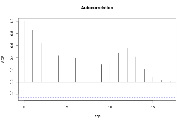
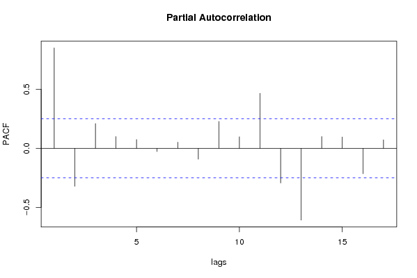
Title produced by software

(Partial) Autocorrelation Function

Date of computation

Wed, 03 Dec 2008 09:32:44 -0700

Cite this page as follows

Statistical Computations at FreeStatistics.org, Office for Research Development and Education, URL https://freestatistics.org/blog/index.php?v=date/2008/Dec/03/t1228322081s3t0rhvdkomstol.htm/, Retrieved Sun, 19 May 2024 07:20:44 +0000

Statistical Computations at FreeStatistics.org, Office for Research Development and Education, URL https://freestatistics.org/blog/index.php?pk=28771, Retrieved Sun, 19 May 2024 07:20:44 +0000

QR Codes:

Paste this QR Code to cite your computation.

Original text written by user:

IsPrivate?

No (this computation is public)

User-defined keywords

Estimated Impact

236

Family? (F = Feedback message, R = changed R code, M = changed R Module, P = changed Parameters, D = changed Data)

-     [Univariate Data Series] [data set] [2008-12-01 19:54:57] [b98453cac15ba1066b407e146608df68]
- RMPD    [(Partial) Autocorrelation Function] [taak 8 werklozen ...] [2008-12-03 16:32:44] [bda7fba231d49184c6a1b627868bbb81] [Current]
-   P       [(Partial) Autocorrelation Function] [taak 8 werklozen ...] [2008-12-03 16:37:45] [e1a46c1dcfccb0cb690f79a1a409b517] 
-   P         [(Partial) Autocorrelation Function] [taak 8 werklozen ...] [2008-12-03 16:39:57] [e1a46c1dcfccb0cb690f79a1a409b517] 
-   P         [(Partial) Autocorrelation Function] [taak 8 werklozen ...] [2008-12-03 16:44:22] [e1a46c1dcfccb0cb690f79a1a409b517] 
- RMP         [Spectral Analysis] [taak 8 werklozen ...] [2008-12-03 16:47:41] [e1a46c1dcfccb0cb690f79a1a409b517] 
-   P           [Spectral Analysis] [taak 8 werklozen ...] [2008-12-03 16:51:44] [e1a46c1dcfccb0cb690f79a1a409b517] 
-   P             [Spectral Analysis] [taak 8 werklozen ...] [2008-12-03 16:54:18] [e1a46c1dcfccb0cb690f79a1a409b517] 
- RMP               [Standard Deviation-Mean Plot] [taak 8 werklozen ...] [2008-12-03 16:58:07] [e1a46c1dcfccb0cb690f79a1a409b517] 
- RM                  [(Partial) Autocorrelation Function] [taak 8 werklozen ...] [2008-12-03 17:08:52] [e1a46c1dcfccb0cb690f79a1a409b517] 
-   P                   [(Partial) Autocorrelation Function] [taak 8 werklozen ...] [2008-12-05 11:44:45] [e1a46c1dcfccb0cb690f79a1a409b517] 
- RMP                     [ARIMA Backward Selection] [taak 8 werklozen ...] [2008-12-05 12:02:13] [e1a46c1dcfccb0cb690f79a1a409b517] 
-   P                       [ARIMA Backward Selection] [taak 8 werklozen ...] [2008-12-08 17:17:01] [e1a46c1dcfccb0cb690f79a1a409b517] 
- RMP                         [Univariate Data Series] [Time plot werkloo...] [2008-12-09 15:43:17] [e1a46c1dcfccb0cb690f79a1a409b517] 
-   P                     [(Partial) Autocorrelation Function] [Paper: Partial au...] [2008-12-13 09:24:08] [e1a46c1dcfccb0cb690f79a1a409b517] 

Feedback Forum

Post a new message

Dataseries X:

Download CSV

Histogram

Boxplots

Summary of computational transaction
Raw Input	view raw input (R code)
Raw Output	view raw output of R engine
Computing time	2 seconds
R Server	'Gwilym Jenkins' @ 72.249.127.135

\begin{tabular}{lllllllll}
\hline
Summary of computational transaction \tabularnewline
Raw Input & view raw input (R code)  \tabularnewline
Raw Output & view raw output of R engine  \tabularnewline
Computing time & 2 seconds \tabularnewline
R Server & 'Gwilym Jenkins' @ 72.249.127.135 \tabularnewline
\hline
\end{tabular}
%Source: https://freestatistics.org/blog/index.php?pk=28771&T=0

[TABLE]
[ROW][C]Summary of computational transaction[/C][/ROW]
[ROW][C]Raw Input[/C][C]view raw input (R code) [/C][/ROW]
[ROW][C]Raw Output[/C][C]view raw output of R engine [/C][/ROW]
[ROW][C]Computing time[/C][C]2 seconds[/C][/ROW]
[ROW][C]R Server[/C][C]'Gwilym Jenkins' @ 72.249.127.135[/C][/ROW]
[/TABLE]
Source: https://freestatistics.org/blog/index.php?pk=28771&T=0

Globally Unique Identifier (entire table): ba.freestatistics.org/blog/index.php?pk=28771&T=0

As an alternative you can also use a QR Code:

The GUIDs for individual cells are displayed in the table below:

Summary of computational transaction
Raw Input	view raw input (R code)
Raw Output	view raw output of R engine
Computing time	2 seconds
R Server	'Gwilym Jenkins' @ 72.249.127.135

Autocorrelation Function
Time lag k	ACF(k)	T-STAT	P-value
1	0.850979	6.6464	0
2	0.635387	4.9625	3e-06
3	0.492618	3.8475	0.000144
4	0.434971	3.3972	0.000602
5	0.422061	3.2964	0.000818
6	0.397862	3.1074	0.001432
7	0.36206	2.8278	0.003166
8	0.302294	2.361	0.010719
9	0.290212	2.2666	0.013485
10	0.336736	2.63	0.005397
11	0.479177	3.7425	0.000203
12	0.560863	4.3805	2.4e-05
13	0.41598	3.2489	0.000943
14	0.212836	1.6623	0.050792
15	0.080756	0.6307	0.265289
16	0.028457	0.2223	0.412429
17	0.013386	0.1045	0.458539

\begin{tabular}{lllllllll}
\hline
Autocorrelation Function \tabularnewline
Time lag k & ACF(k) & T-STAT & P-value \tabularnewline
1 & 0.850979 & 6.6464 & 0 \tabularnewline
2 & 0.635387 & 4.9625 & 3e-06 \tabularnewline
3 & 0.492618 & 3.8475 & 0.000144 \tabularnewline
4 & 0.434971 & 3.3972 & 0.000602 \tabularnewline
5 & 0.422061 & 3.2964 & 0.000818 \tabularnewline
6 & 0.397862 & 3.1074 & 0.001432 \tabularnewline
7 & 0.36206 & 2.8278 & 0.003166 \tabularnewline
8 & 0.302294 & 2.361 & 0.010719 \tabularnewline
9 & 0.290212 & 2.2666 & 0.013485 \tabularnewline
10 & 0.336736 & 2.63 & 0.005397 \tabularnewline
11 & 0.479177 & 3.7425 & 0.000203 \tabularnewline
12 & 0.560863 & 4.3805 & 2.4e-05 \tabularnewline
13 & 0.41598 & 3.2489 & 0.000943 \tabularnewline
14 & 0.212836 & 1.6623 & 0.050792 \tabularnewline
15 & 0.080756 & 0.6307 & 0.265289 \tabularnewline
16 & 0.028457 & 0.2223 & 0.412429 \tabularnewline
17 & 0.013386 & 0.1045 & 0.458539 \tabularnewline
\hline
\end{tabular}
%Source: https://freestatistics.org/blog/index.php?pk=28771&T=1

[TABLE]
[ROW][C]Autocorrelation Function[/C][/ROW]
[ROW][C]Time lag k[/C][C]ACF(k)[/C][C]T-STAT[/C][C]P-value[/C][/ROW]
[ROW][C]1[/C][C]0.850979[/C][C]6.6464[/C][C]0[/C][/ROW]
[ROW][C]2[/C][C]0.635387[/C][C]4.9625[/C][C]3e-06[/C][/ROW]
[ROW][C]3[/C][C]0.492618[/C][C]3.8475[/C][C]0.000144[/C][/ROW]
[ROW][C]4[/C][C]0.434971[/C][C]3.3972[/C][C]0.000602[/C][/ROW]
[ROW][C]5[/C][C]0.422061[/C][C]3.2964[/C][C]0.000818[/C][/ROW]
[ROW][C]6[/C][C]0.397862[/C][C]3.1074[/C][C]0.001432[/C][/ROW]
[ROW][C]7[/C][C]0.36206[/C][C]2.8278[/C][C]0.003166[/C][/ROW]
[ROW][C]8[/C][C]0.302294[/C][C]2.361[/C][C]0.010719[/C][/ROW]
[ROW][C]9[/C][C]0.290212[/C][C]2.2666[/C][C]0.013485[/C][/ROW]
[ROW][C]10[/C][C]0.336736[/C][C]2.63[/C][C]0.005397[/C][/ROW]
[ROW][C]11[/C][C]0.479177[/C][C]3.7425[/C][C]0.000203[/C][/ROW]
[ROW][C]12[/C][C]0.560863[/C][C]4.3805[/C][C]2.4e-05[/C][/ROW]
[ROW][C]13[/C][C]0.41598[/C][C]3.2489[/C][C]0.000943[/C][/ROW]
[ROW][C]14[/C][C]0.212836[/C][C]1.6623[/C][C]0.050792[/C][/ROW]
[ROW][C]15[/C][C]0.080756[/C][C]0.6307[/C][C]0.265289[/C][/ROW]
[ROW][C]16[/C][C]0.028457[/C][C]0.2223[/C][C]0.412429[/C][/ROW]
[ROW][C]17[/C][C]0.013386[/C][C]0.1045[/C][C]0.458539[/C][/ROW]
[/TABLE]
Source: https://freestatistics.org/blog/index.php?pk=28771&T=1

Globally Unique Identifier (entire table): ba.freestatistics.org/blog/index.php?pk=28771&T=1

As an alternative you can also use a QR Code:

The GUIDs for individual cells are displayed in the table below:

Autocorrelation Function
Time lag k	ACF(k)	T-STAT	P-value
1	0.850979	6.6464	0
2	0.635387	4.9625	3e-06
3	0.492618	3.8475	0.000144
4	0.434971	3.3972	0.000602
5	0.422061	3.2964	0.000818
6	0.397862	3.1074	0.001432
7	0.36206	2.8278	0.003166
8	0.302294	2.361	0.010719
9	0.290212	2.2666	0.013485
10	0.336736	2.63	0.005397
11	0.479177	3.7425	0.000203
12	0.560863	4.3805	2.4e-05
13	0.41598	3.2489	0.000943
14	0.212836	1.6623	0.050792
15	0.080756	0.6307	0.265289
16	0.028457	0.2223	0.412429
17	0.013386	0.1045	0.458539

Partial Autocorrelation Function
Time lag k	PACF(k)	T-STAT	P-value
1	0.850979	6.6464	0
2	-0.321855	-2.5138	0.0073
3	0.209418	1.6356	0.053536
4	0.099845	0.7798	0.219259
5	0.074091	0.5787	0.282471
6	-0.02757	-0.2153	0.415116
7	0.051836	0.4049	0.3435
8	-0.092606	-0.7233	0.236137
9	0.227513	1.7769	0.040283
10	0.097405	0.7608	0.224866
11	0.466023	3.6398	0.000282
12	-0.294016	-2.2963	0.012553
13	-0.608435	-4.752	6e-06
14	0.100049	0.7814	0.218793
15	0.095809	0.7483	0.22858
16	-0.215232	-1.681	0.048937
17	0.071697	0.56	0.288776

\begin{tabular}{lllllllll}
\hline
Partial Autocorrelation Function \tabularnewline
Time lag k & PACF(k) & T-STAT & P-value \tabularnewline
1 & 0.850979 & 6.6464 & 0 \tabularnewline
2 & -0.321855 & -2.5138 & 0.0073 \tabularnewline
3 & 0.209418 & 1.6356 & 0.053536 \tabularnewline
4 & 0.099845 & 0.7798 & 0.219259 \tabularnewline
5 & 0.074091 & 0.5787 & 0.282471 \tabularnewline
6 & -0.02757 & -0.2153 & 0.415116 \tabularnewline
7 & 0.051836 & 0.4049 & 0.3435 \tabularnewline
8 & -0.092606 & -0.7233 & 0.236137 \tabularnewline
9 & 0.227513 & 1.7769 & 0.040283 \tabularnewline
10 & 0.097405 & 0.7608 & 0.224866 \tabularnewline
11 & 0.466023 & 3.6398 & 0.000282 \tabularnewline
12 & -0.294016 & -2.2963 & 0.012553 \tabularnewline
13 & -0.608435 & -4.752 & 6e-06 \tabularnewline
14 & 0.100049 & 0.7814 & 0.218793 \tabularnewline
15 & 0.095809 & 0.7483 & 0.22858 \tabularnewline
16 & -0.215232 & -1.681 & 0.048937 \tabularnewline
17 & 0.071697 & 0.56 & 0.288776 \tabularnewline
\hline
\end{tabular}
%Source: https://freestatistics.org/blog/index.php?pk=28771&T=2

[TABLE]
[ROW][C]Partial Autocorrelation Function[/C][/ROW]
[ROW][C]Time lag k[/C][C]PACF(k)[/C][C]T-STAT[/C][C]P-value[/C][/ROW]
[ROW][C]1[/C][C]0.850979[/C][C]6.6464[/C][C]0[/C][/ROW]
[ROW][C]2[/C][C]-0.321855[/C][C]-2.5138[/C][C]0.0073[/C][/ROW]
[ROW][C]3[/C][C]0.209418[/C][C]1.6356[/C][C]0.053536[/C][/ROW]
[ROW][C]4[/C][C]0.099845[/C][C]0.7798[/C][C]0.219259[/C][/ROW]
[ROW][C]5[/C][C]0.074091[/C][C]0.5787[/C][C]0.282471[/C][/ROW]
[ROW][C]6[/C][C]-0.02757[/C][C]-0.2153[/C][C]0.415116[/C][/ROW]
[ROW][C]7[/C][C]0.051836[/C][C]0.4049[/C][C]0.3435[/C][/ROW]
[ROW][C]8[/C][C]-0.092606[/C][C]-0.7233[/C][C]0.236137[/C][/ROW]
[ROW][C]9[/C][C]0.227513[/C][C]1.7769[/C][C]0.040283[/C][/ROW]
[ROW][C]10[/C][C]0.097405[/C][C]0.7608[/C][C]0.224866[/C][/ROW]
[ROW][C]11[/C][C]0.466023[/C][C]3.6398[/C][C]0.000282[/C][/ROW]
[ROW][C]12[/C][C]-0.294016[/C][C]-2.2963[/C][C]0.012553[/C][/ROW]
[ROW][C]13[/C][C]-0.608435[/C][C]-4.752[/C][C]6e-06[/C][/ROW]
[ROW][C]14[/C][C]0.100049[/C][C]0.7814[/C][C]0.218793[/C][/ROW]
[ROW][C]15[/C][C]0.095809[/C][C]0.7483[/C][C]0.22858[/C][/ROW]
[ROW][C]16[/C][C]-0.215232[/C][C]-1.681[/C][C]0.048937[/C][/ROW]
[ROW][C]17[/C][C]0.071697[/C][C]0.56[/C][C]0.288776[/C][/ROW]
[/TABLE]
Source: https://freestatistics.org/blog/index.php?pk=28771&T=2

Globally Unique Identifier (entire table): ba.freestatistics.org/blog/index.php?pk=28771&T=2

As an alternative you can also use a QR Code:

The GUIDs for individual cells are displayed in the table below:

Partial Autocorrelation Function
Time lag k	PACF(k)	T-STAT	P-value
1	0.850979	6.6464	0
2	-0.321855	-2.5138	0.0073
3	0.209418	1.6356	0.053536
4	0.099845	0.7798	0.219259
5	0.074091	0.5787	0.282471
6	-0.02757	-0.2153	0.415116
7	0.051836	0.4049	0.3435
8	-0.092606	-0.7233	0.236137
9	0.227513	1.7769	0.040283
10	0.097405	0.7608	0.224866
11	0.466023	3.6398	0.000282
12	-0.294016	-2.2963	0.012553
13	-0.608435	-4.752	6e-06
14	0.100049	0.7814	0.218793
15	0.095809	0.7483	0.22858
16	-0.215232	-1.681	0.048937
17	0.071697	0.56	0.288776

Figure 1

PNG link

Postscript link

PDF link

Figure 2

PNG link

Postscript link

PDF link

Parameters (Session):

par1 = Default ; par2 = 1 ; par3 = 0 ; par4 = 0 ; par5 = 12 ;

Parameters (R input):

par1 = Default ; par2 = 1 ; par3 = 0 ; par4 = 0 ; par5 = 12 ;

R code (references can be found in the software module):

if (par1 == 'Default') {
par1 = 10*log10(length(x))
} else {
par1 <- as.numeric(par1)
}
par2 <- as.numeric(par2)
par3 <- as.numeric(par3)
par4 <- as.numeric(par4)
par5 <- as.numeric(par5)
if (par2 == 0) {
x <- log(x)
} else {
x <- (x ^ par2 - 1) / par2
}
if (par3 > 0) x <- diff(x,lag=1,difference=par3)
if (par4 > 0) x <- diff(x,lag=par5,difference=par4)
bitmap(file='pic1.png')
racf <- acf(x,par1,main='Autocorrelation',xlab='lags',ylab='ACF')
dev.off()
bitmap(file='pic2.png')
rpacf <- pacf(x,par1,main='Partial Autocorrelation',xlab='lags',ylab='PACF')
dev.off()
(myacf <- c(racf$acf))
(mypacf <- c(rpacf$acf))
lengthx <- length(x)
sqrtn <- sqrt(lengthx)
load(file='createtable')
a<-table.start()
a<-table.row.start(a)
a<-table.element(a,'Autocorrelation Function',4,TRUE)
a<-table.row.end(a)
a<-table.row.start(a)
a<-table.element(a,'Time lag k',header=TRUE)
a<-table.element(a,hyperlink('basics.htm','ACF(k)','click here for more information about the Autocorrelation Function'),header=TRUE)
a<-table.element(a,'T-STAT',header=TRUE)
a<-table.element(a,'P-value',header=TRUE)
a<-table.row.end(a)
for (i in 2:(par1+1)) {
a<-table.row.start(a)
a<-table.element(a,i-1,header=TRUE)
a<-table.element(a,round(myacf[i],6))
mytstat <- myacf[i]*sqrtn
a<-table.element(a,round(mytstat,4))
a<-table.element(a,round(1-pt(abs(mytstat),lengthx),6))
a<-table.row.end(a)
}
a<-table.end(a)
table.save(a,file='mytable.tab')
a<-table.start()
a<-table.row.start(a)
a<-table.element(a,'Partial Autocorrelation Function',4,TRUE)
a<-table.row.end(a)
a<-table.row.start(a)
a<-table.element(a,'Time lag k',header=TRUE)
a<-table.element(a,hyperlink('basics.htm','PACF(k)','click here for more information about the Partial Autocorrelation Function'),header=TRUE)
a<-table.element(a,'T-STAT',header=TRUE)
a<-table.element(a,'P-value',header=TRUE)
a<-table.row.end(a)
for (i in 1:par1) {
a<-table.row.start(a)
a<-table.element(a,i,header=TRUE)
a<-table.element(a,round(mypacf[i],6))
mytstat <- mypacf[i]*sqrtn
a<-table.element(a,round(mytstat,4))
a<-table.element(a,round(1-pt(abs(mytstat),lengthx),6))
a<-table.row.end(a)
}
a<-table.end(a)
table.save(a,file='mytable1.tab')

Free Statistics

Description of Statistical Computation

Tree of Dependent Computations

Dataset

Tables (Output of Computation)

Figures (Output of Computation)

Input Parameters & R Code