Free Statistics

of Irreproducible Research!

Author's title

Author*Unverified author*
R Software Modulerwasp_cross.wasp
Title produced by softwareCross Correlation Function
Date of computationWed, 03 Dec 2008 03:40:20 -0700
Cite this page as followsStatistical Computations at FreeStatistics.org, Office for Research Development and Education, URL https://freestatistics.org/blog/index.php?v=date/2008/Dec/03/t1228301005nkv3pfs71bz0o4y.htm/, Retrieved Sun, 19 May 2024 07:18:27 +0000
Statistical Computations at FreeStatistics.org, Office for Research Development and Education, URL https://freestatistics.org/blog/index.php?pk=28608, Retrieved Sun, 19 May 2024 07:18:27 +0000
QR Codes:

Original text written by user:
IsPrivate?No (this computation is public)
User-defined keywords
Estimated Impact175
Family? (F = Feedback message, R = changed R code, M = changed R Module, P = changed Parameters, D = changed Data)
F       [Cross Correlation Function] [] [2008-12-03 10:40:20] [ed75e673b8609ce7f7795f94157397be] [Current]
Feedback Forum
2008-12-06 13:03:43 [Nicolaj Wuyts] [reply
Deze vraag is correct beantwoord door de student
2008-12-07 19:30:57 [Jasmine Hendrikx] [reply
Evaluatie Q9:
De cross correlatiefunctie na transformatie van de tijdreeksen is goed berekend (de lambda is wel gelijkgesteld aan 1, omdat de student de optimale lambda niet berekend heeft in Q8).De bespreking is ook goed. Het is inderdaad zo dat er nu een opvallend verschil is. Alle coëfficiënten liggen nu binnen het betrouwbaarheidsinterval en zijn niet meer significant verschillend van 0. Hieruit kun je inderdaad concluderen dat de verleden, de huidige en toekomstige waarden van Xt geen invloed hebben op Yt. Voor de transformatie waren er zowel links als rechts van k=0 veel significante verschillen (simultaan effect).
Na de transformatie zijn deze significante verschillen in grote mate verdwenen. Dit is een typisch fenomeen. Na transformatie zie je meestal ofwel niets meer of véél minder significante verschillen. De verklaring hiervoor is terug te vinden in partiële correlatie. De correlatie tussen Xt enYt kan vertekend worden indien er een andere variabele is die zowel Yt als Xt sterk beïnvloedt. Zt is dus duidelijk aanwezig in de 2 tijdreeksen. De 2 reeksen vertonen dezelfde trend. Er is autocorrelatie bij de twee reeksen aanwezig. Als we de trend uit X en Y halen, zullen we dus een veel zuiverder beeld zien. Q9 geeft dus een veel betrouwbaarder beeld dan Q7. We kunnen dus eigenlijk spreken van een nonsenscorrelatie tussen Xt en Yt, zoals de student ook terecht vermeldt.

Post a new message
Dataseries X:
101.2
100.5
98
106.6
90.1
96.9
125.9
112
100
123.9
79.8
83.4
113.6
112.9
104
109.9
99
106.3
128.9
111.1
102.9
130
87
87.5
117.6
103.4
110.8
112.6
102.5
112.4
135.6
105.1
127.7
137
91
90.5
122.4
123.3
124.3
120
118.1
119
142.7
123.6
129.6
151.6
110.4
99.2
130.5
136.2
129.7
128
121.6
135.8
143.8
147.5
136.2
156.6
123.3
104.5
143.6
Dataseries Y:
6.8
6.9
6.8
6.2
6.2
6.6
6.8
7.1
7.3
7.2
7
7
7
7.3
7.5
7.2
7.7
8
7.9
8
8
7.9
7.9
7.9
8.1
8.1
8.2
8.1
8.3
8.5
8.6
8.7
8.7
8.5
8.4
8.5
8.8
8.7
8.6
8
8.1
8.2
8.6
8.6
8.5
8.3
8.2
8.7
9.3
9.3
8.8
7.5
7.2
7.5
8.3
8.8
8.9
8.6
8.4
8.4
8.4


Summary of computational transaction
Raw Inputview raw input (R code)
Raw Outputview raw output of R engine
Computing time3 seconds
R Server'Herman Ole Andreas Wold' @ 193.190.124.10:1001

\begin{tabular}{lllllllll}
\hline
Summary of computational transaction \tabularnewline
Raw Input & view raw input (R code)  \tabularnewline
Raw Output & view raw output of R engine  \tabularnewline
Computing time & 3 seconds \tabularnewline
R Server & 'Herman Ole Andreas Wold' @ 193.190.124.10:1001 \tabularnewline
\hline
\end{tabular}
%Source: https://freestatistics.org/blog/index.php?pk=28608&T=0

[TABLE]
[ROW][C]Summary of computational transaction[/C][/ROW]
[ROW][C]Raw Input[/C][C]view raw input (R code) [/C][/ROW]
[ROW][C]Raw Output[/C][C]view raw output of R engine [/C][/ROW]
[ROW][C]Computing time[/C][C]3 seconds[/C][/ROW]
[ROW][C]R Server[/C][C]'Herman Ole Andreas Wold' @ 193.190.124.10:1001[/C][/ROW]
[/TABLE]
Source: https://freestatistics.org/blog/index.php?pk=28608&T=0

Globally Unique Identifier (entire table): ba.freestatistics.org/blog/index.php?pk=28608&T=0

As an alternative you can also use a QR Code:  

The GUIDs for individual cells are displayed in the table below:

Summary of computational transaction
Raw Inputview raw input (R code)
Raw Outputview raw output of R engine
Computing time3 seconds
R Server'Herman Ole Andreas Wold' @ 193.190.124.10:1001


Cross Correlation Function
ParameterValue
Box-Cox transformation parameter (lambda) of X series1
Degree of non-seasonal differencing (d) of X series0
Degree of seasonal differencing (D) of X series1
Seasonal Period (s)12
Box-Cox transformation parameter (lambda) of Y series1
Degree of non-seasonal differencing (d) of Y series1
Degree of seasonal differencing (D) of Y series0
krho(Y[t],X[t+k])
-130.0548039609355481
-12-0.0839378831388449
-11-0.0351035937172314
-10-0.0208002216639106
-9-0.0714604574745187
-8-0.0468417667866732
-7-0.0119972498944033
-60.0455230695078016
-5-0.0735278078136222
-4-0.0130858237815814
-30.0461058983593123
-2-0.132736450792141
-1-0.0564227210682937
0-0.0472230496611453
1-0.110831486440655
20.127452261211308
3-0.187427230124912
40.0684707334755717
50.083223447772476
6-0.0551374894460575
7-0.060186291374603
8-0.0110342662242612
9-0.0404881802679695
100.0745513304805988
11-0.0193976722341444
12-0.0431056458391769
130.14309087536251

\begin{tabular}{lllllllll}
\hline
Cross Correlation Function \tabularnewline
Parameter & Value \tabularnewline
Box-Cox transformation parameter (lambda) of X series & 1 \tabularnewline
Degree of non-seasonal differencing (d) of X series & 0 \tabularnewline
Degree of seasonal differencing (D) of X series & 1 \tabularnewline
Seasonal Period (s) & 12 \tabularnewline
Box-Cox transformation parameter (lambda) of Y series & 1 \tabularnewline
Degree of non-seasonal differencing (d) of Y series & 1 \tabularnewline
Degree of seasonal differencing (D) of Y series & 0 \tabularnewline
k & rho(Y[t],X[t+k]) \tabularnewline
-13 & 0.0548039609355481 \tabularnewline
-12 & -0.0839378831388449 \tabularnewline
-11 & -0.0351035937172314 \tabularnewline
-10 & -0.0208002216639106 \tabularnewline
-9 & -0.0714604574745187 \tabularnewline
-8 & -0.0468417667866732 \tabularnewline
-7 & -0.0119972498944033 \tabularnewline
-6 & 0.0455230695078016 \tabularnewline
-5 & -0.0735278078136222 \tabularnewline
-4 & -0.0130858237815814 \tabularnewline
-3 & 0.0461058983593123 \tabularnewline
-2 & -0.132736450792141 \tabularnewline
-1 & -0.0564227210682937 \tabularnewline
0 & -0.0472230496611453 \tabularnewline
1 & -0.110831486440655 \tabularnewline
2 & 0.127452261211308 \tabularnewline
3 & -0.187427230124912 \tabularnewline
4 & 0.0684707334755717 \tabularnewline
5 & 0.083223447772476 \tabularnewline
6 & -0.0551374894460575 \tabularnewline
7 & -0.060186291374603 \tabularnewline
8 & -0.0110342662242612 \tabularnewline
9 & -0.0404881802679695 \tabularnewline
10 & 0.0745513304805988 \tabularnewline
11 & -0.0193976722341444 \tabularnewline
12 & -0.0431056458391769 \tabularnewline
13 & 0.14309087536251 \tabularnewline
\hline
\end{tabular}
%Source: https://freestatistics.org/blog/index.php?pk=28608&T=1

[TABLE]
[ROW][C]Cross Correlation Function[/C][/ROW]
[ROW][C]Parameter[/C][C]Value[/C][/ROW]
[ROW][C]Box-Cox transformation parameter (lambda) of X series[/C][C]1[/C][/ROW]
[ROW][C]Degree of non-seasonal differencing (d) of X series[/C][C]0[/C][/ROW]
[ROW][C]Degree of seasonal differencing (D) of X series[/C][C]1[/C][/ROW]
[ROW][C]Seasonal Period (s)[/C][C]12[/C][/ROW]
[ROW][C]Box-Cox transformation parameter (lambda) of Y series[/C][C]1[/C][/ROW]
[ROW][C]Degree of non-seasonal differencing (d) of Y series[/C][C]1[/C][/ROW]
[ROW][C]Degree of seasonal differencing (D) of Y series[/C][C]0[/C][/ROW]
[ROW][C]k[/C][C]rho(Y[t],X[t+k])[/C][/ROW]
[ROW][C]-13[/C][C]0.0548039609355481[/C][/ROW]
[ROW][C]-12[/C][C]-0.0839378831388449[/C][/ROW]
[ROW][C]-11[/C][C]-0.0351035937172314[/C][/ROW]
[ROW][C]-10[/C][C]-0.0208002216639106[/C][/ROW]
[ROW][C]-9[/C][C]-0.0714604574745187[/C][/ROW]
[ROW][C]-8[/C][C]-0.0468417667866732[/C][/ROW]
[ROW][C]-7[/C][C]-0.0119972498944033[/C][/ROW]
[ROW][C]-6[/C][C]0.0455230695078016[/C][/ROW]
[ROW][C]-5[/C][C]-0.0735278078136222[/C][/ROW]
[ROW][C]-4[/C][C]-0.0130858237815814[/C][/ROW]
[ROW][C]-3[/C][C]0.0461058983593123[/C][/ROW]
[ROW][C]-2[/C][C]-0.132736450792141[/C][/ROW]
[ROW][C]-1[/C][C]-0.0564227210682937[/C][/ROW]
[ROW][C]0[/C][C]-0.0472230496611453[/C][/ROW]
[ROW][C]1[/C][C]-0.110831486440655[/C][/ROW]
[ROW][C]2[/C][C]0.127452261211308[/C][/ROW]
[ROW][C]3[/C][C]-0.187427230124912[/C][/ROW]
[ROW][C]4[/C][C]0.0684707334755717[/C][/ROW]
[ROW][C]5[/C][C]0.083223447772476[/C][/ROW]
[ROW][C]6[/C][C]-0.0551374894460575[/C][/ROW]
[ROW][C]7[/C][C]-0.060186291374603[/C][/ROW]
[ROW][C]8[/C][C]-0.0110342662242612[/C][/ROW]
[ROW][C]9[/C][C]-0.0404881802679695[/C][/ROW]
[ROW][C]10[/C][C]0.0745513304805988[/C][/ROW]
[ROW][C]11[/C][C]-0.0193976722341444[/C][/ROW]
[ROW][C]12[/C][C]-0.0431056458391769[/C][/ROW]
[ROW][C]13[/C][C]0.14309087536251[/C][/ROW]
[/TABLE]
Source: https://freestatistics.org/blog/index.php?pk=28608&T=1

Globally Unique Identifier (entire table): ba.freestatistics.org/blog/index.php?pk=28608&T=1

As an alternative you can also use a QR Code:  

The GUIDs for individual cells are displayed in the table below:

Cross Correlation Function
ParameterValue
Box-Cox transformation parameter (lambda) of X series1
Degree of non-seasonal differencing (d) of X series0
Degree of seasonal differencing (D) of X series1
Seasonal Period (s)12
Box-Cox transformation parameter (lambda) of Y series1
Degree of non-seasonal differencing (d) of Y series1
Degree of seasonal differencing (D) of Y series0
krho(Y[t],X[t+k])
-130.0548039609355481
-12-0.0839378831388449
-11-0.0351035937172314
-10-0.0208002216639106
-9-0.0714604574745187
-8-0.0468417667866732
-7-0.0119972498944033
-60.0455230695078016
-5-0.0735278078136222
-4-0.0130858237815814
-30.0461058983593123
-2-0.132736450792141
-1-0.0564227210682937
0-0.0472230496611453
1-0.110831486440655
20.127452261211308
3-0.187427230124912
40.0684707334755717
50.083223447772476
6-0.0551374894460575
7-0.060186291374603
8-0.0110342662242612
9-0.0404881802679695
100.0745513304805988
11-0.0193976722341444
12-0.0431056458391769
130.14309087536251


Parameters (Session):
par1 = 1 ; par2 = 0 ; par3 = 0 ; par4 = 12 ;
Parameters (R input):
par1 = 1 ; par2 = 0 ; par3 = 1 ; par4 = 12 ; par5 = 1 ; par6 = 1 ; par7 = 0 ;
R code (references can be found in the software module):
par1 <- as.numeric(par1)
par2 <- as.numeric(par2)
par3 <- as.numeric(par3)
par4 <- as.numeric(par4)
par5 <- as.numeric(par5)
par6 <- as.numeric(par6)
par7 <- as.numeric(par7)
if (par1 == 0) {
x <- log(x)
} else {
x <- (x ^ par1 - 1) / par1
}
if (par5 == 0) {
y <- log(y)
} else {
y <- (y ^ par5 - 1) / par5
}
if (par2 > 0) x <- diff(x,lag=1,difference=par2)
if (par6 > 0) y <- diff(y,lag=1,difference=par6)
if (par3 > 0) x <- diff(x,lag=par4,difference=par3)
if (par7 > 0) y <- diff(y,lag=par4,difference=par7)
x
y
bitmap(file='test1.png')
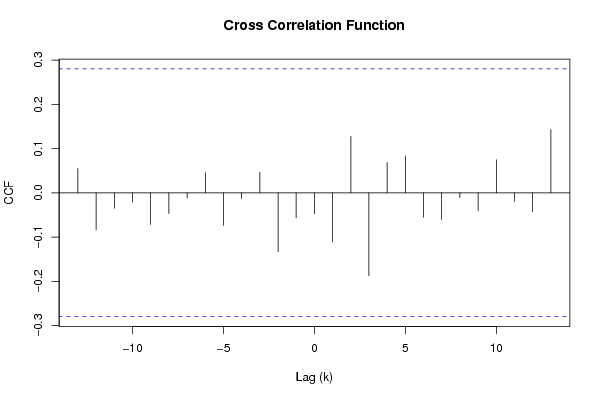
(r <- ccf(x,y,main='Cross Correlation Function',ylab='CCF',xlab='Lag (k)'))
dev.off()
load(file='createtable')
a<-table.start()
a<-table.row.start(a)
a<-table.element(a,'Cross Correlation Function',2,TRUE)
a<-table.row.end(a)
a<-table.row.start(a)
a<-table.element(a,'Parameter',header=TRUE)
a<-table.element(a,'Value',header=TRUE)
a<-table.row.end(a)
a<-table.row.start(a)
a<-table.element(a,'Box-Cox transformation parameter (lambda) of X series',header=TRUE)
a<-table.element(a,par1)
a<-table.row.end(a)
a<-table.row.start(a)
a<-table.element(a,'Degree of non-seasonal differencing (d) of X series',header=TRUE)
a<-table.element(a,par2)
a<-table.row.end(a)
a<-table.row.start(a)
a<-table.element(a,'Degree of seasonal differencing (D) of X series',header=TRUE)
a<-table.element(a,par3)
a<-table.row.end(a)
a<-table.row.start(a)
a<-table.element(a,'Seasonal Period (s)',header=TRUE)
a<-table.element(a,par4)
a<-table.row.end(a)
a<-table.row.start(a)
a<-table.element(a,'Box-Cox transformation parameter (lambda) of Y series',header=TRUE)
a<-table.element(a,par5)
a<-table.row.end(a)
a<-table.row.start(a)
a<-table.element(a,'Degree of non-seasonal differencing (d) of Y series',header=TRUE)
a<-table.element(a,par6)
a<-table.row.end(a)
a<-table.row.start(a)
a<-table.element(a,'Degree of seasonal differencing (D) of Y series',header=TRUE)
a<-table.element(a,par7)
a<-table.row.end(a)
a<-table.row.start(a)
a<-table.element(a,'k',header=TRUE)
a<-table.element(a,'rho(Y[t],X[t+k])',header=TRUE)
a<-table.row.end(a)
mylength <- length(r$acf)
myhalf <- floor((mylength-1)/2)
for (i in 1:mylength) {
a<-table.row.start(a)
a<-table.element(a,i-myhalf-1,header=TRUE)
a<-table.element(a,r$acf[i])
a<-table.row.end(a)
}
a<-table.end(a)
table.save(a,file='mytable.tab')