Repository of Reproducible Computations

Free Statistics

of Irreproducible Research!

Author's title

Author

*Unverified author*

R Software Module

rwasp_autocorrelation.wasp

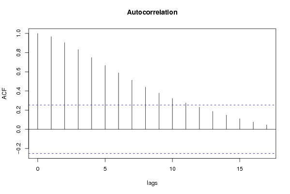
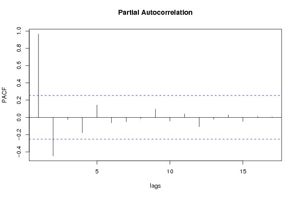
Title produced by software

(Partial) Autocorrelation Function

Date of computation

Wed, 03 Dec 2008 00:40:58 -0700

Cite this page as follows

Statistical Computations at FreeStatistics.org, Office for Research Development and Education, URL https://freestatistics.org/blog/index.php?v=date/2008/Dec/03/t1228290126bo1tmok4sj32atf.htm/, Retrieved Sun, 19 May 2024 07:07:21 +0000

Statistical Computations at FreeStatistics.org, Office for Research Development and Education, URL https://freestatistics.org/blog/index.php?pk=28552, Retrieved Sun, 19 May 2024 07:07:21 +0000

QR Codes:

Paste this QR Code to cite your computation.

Original text written by user:

IsPrivate?

No (this computation is public)

User-defined keywords

Estimated Impact

217

Family? (F = Feedback message, R = changed R code, M = changed R Module, P = changed Parameters, D = changed Data)

F       [(Partial) Autocorrelation Function] [] [2008-12-03 07:40:58] [e02910eed3830f1815f587e12f46cbdb] [Current]
-   PD    [(Partial) Autocorrelation Function] [] [2008-12-06 11:35:59] [996314793dac993597edc1ca2281ff39] 

Feedback Forum

2008-12-06 10:57:12 [Angelique Van de Vijver] [reply] 
goede berekening en juiste vaststellingen van de student, wel weinig uitleg.  
We zien op de ACF inderdaad een langzaam dalend patroon wat dus op een langetermijntrend wijst. We zien hier een positieve autocorrelatie : Het verleden van de reeks geeft ons informatie over de daaropvolgende waarden. Waarden worden bepaald door het verleden( als de vorige waarde groot is, zal de huidige waarde ook groot zijn). We zien ook dat de meeste balkjes zich boven het 95% betrouwbaarheidsinterval bevinden en dus significant verschillend van 0 zijn. De laatste balkjes vallen onder het betrouwbaarheidsinterval en zijn dus niet significant verschillend van 0. 
Hier moeten we niet-seizoenaal differentieren om zo tot een stationaire tijdreeks te komen.
2008-12-06 11:41:09 [Angelique Van de Vijver] [reply] 
Student heeft wel een verkeerde berekening gemaakt, merk ik nu op. Number of time lags stond bij haar op default. Ik heb de berekening opnieuw gemaakt met number of time lags gelijk aan 36: 
http://www.freestatistics.org/blog/date/2008/Dec/06/t1228563476sucjulrt1w2cl7d.htm 
Nu krijgen we wel een andere ACF. Er is wel nog altijd een langzaam dalend verloop en dus een langetermijntrend. We moeten dus nog altijd niet-seizoenaal differentiëren om deze tren eruit te halen.

Post a new message

Dataseries X:

Download CSV

Histogram

Boxplots

Summary of computational transaction
Raw Input	view raw input (R code)
Raw Output	view raw output of R engine
Computing time	0 seconds
R Server	'Gwilym Jenkins' @ 72.249.127.135

\begin{tabular}{lllllllll}
\hline
Summary of computational transaction \tabularnewline
Raw Input & view raw input (R code)  \tabularnewline
Raw Output & view raw output of R engine  \tabularnewline
Computing time & 0 seconds \tabularnewline
R Server & 'Gwilym Jenkins' @ 72.249.127.135 \tabularnewline
\hline
\end{tabular}
%Source: https://freestatistics.org/blog/index.php?pk=28552&T=0

[TABLE]
[ROW][C]Summary of computational transaction[/C][/ROW]
[ROW][C]Raw Input[/C][C]view raw input (R code) [/C][/ROW]
[ROW][C]Raw Output[/C][C]view raw output of R engine [/C][/ROW]
[ROW][C]Computing time[/C][C]0 seconds[/C][/ROW]
[ROW][C]R Server[/C][C]'Gwilym Jenkins' @ 72.249.127.135[/C][/ROW]
[/TABLE]
Source: https://freestatistics.org/blog/index.php?pk=28552&T=0

Globally Unique Identifier (entire table): ba.freestatistics.org/blog/index.php?pk=28552&T=0

As an alternative you can also use a QR Code:

The GUIDs for individual cells are displayed in the table below:

Summary of computational transaction
Raw Input	view raw input (R code)
Raw Output	view raw output of R engine
Computing time	0 seconds
R Server	'Gwilym Jenkins' @ 72.249.127.135

Autocorrelation Function
Time lag k	ACF(k)	T-STAT	P-value
1	0.966547	7.4868	0
2	0.90477	7.0083	0
3	0.831977	6.4445	0
4	0.747844	5.7928	0
5	0.666305	5.1612	1e-06
6	0.589038	4.5627	1.3e-05
7	0.512466	3.9695	9.8e-05
8	0.440078	3.4088	0.000586
9	0.377672	2.9254	0.002425
10	0.321984	2.4941	0.007701
11	0.274388	2.1254	0.01884
12	0.230962	1.789	0.039329
13	0.18759	1.4531	0.075708
14	0.148365	1.1492	0.127511
15	0.110932	0.8593	0.196805
16	0.076007	0.5887	0.27912
17	0.046245	0.3582	0.36072

\begin{tabular}{lllllllll}
\hline
Autocorrelation Function \tabularnewline
Time lag k & ACF(k) & T-STAT & P-value \tabularnewline
1 & 0.966547 & 7.4868 & 0 \tabularnewline
2 & 0.90477 & 7.0083 & 0 \tabularnewline
3 & 0.831977 & 6.4445 & 0 \tabularnewline
4 & 0.747844 & 5.7928 & 0 \tabularnewline
5 & 0.666305 & 5.1612 & 1e-06 \tabularnewline
6 & 0.589038 & 4.5627 & 1.3e-05 \tabularnewline
7 & 0.512466 & 3.9695 & 9.8e-05 \tabularnewline
8 & 0.440078 & 3.4088 & 0.000586 \tabularnewline
9 & 0.377672 & 2.9254 & 0.002425 \tabularnewline
10 & 0.321984 & 2.4941 & 0.007701 \tabularnewline
11 & 0.274388 & 2.1254 & 0.01884 \tabularnewline
12 & 0.230962 & 1.789 & 0.039329 \tabularnewline
13 & 0.18759 & 1.4531 & 0.075708 \tabularnewline
14 & 0.148365 & 1.1492 & 0.127511 \tabularnewline
15 & 0.110932 & 0.8593 & 0.196805 \tabularnewline
16 & 0.076007 & 0.5887 & 0.27912 \tabularnewline
17 & 0.046245 & 0.3582 & 0.36072 \tabularnewline
\hline
\end{tabular}
%Source: https://freestatistics.org/blog/index.php?pk=28552&T=1

[TABLE]
[ROW][C]Autocorrelation Function[/C][/ROW]
[ROW][C]Time lag k[/C][C]ACF(k)[/C][C]T-STAT[/C][C]P-value[/C][/ROW]
[ROW][C]1[/C][C]0.966547[/C][C]7.4868[/C][C]0[/C][/ROW]
[ROW][C]2[/C][C]0.90477[/C][C]7.0083[/C][C]0[/C][/ROW]
[ROW][C]3[/C][C]0.831977[/C][C]6.4445[/C][C]0[/C][/ROW]
[ROW][C]4[/C][C]0.747844[/C][C]5.7928[/C][C]0[/C][/ROW]
[ROW][C]5[/C][C]0.666305[/C][C]5.1612[/C][C]1e-06[/C][/ROW]
[ROW][C]6[/C][C]0.589038[/C][C]4.5627[/C][C]1.3e-05[/C][/ROW]
[ROW][C]7[/C][C]0.512466[/C][C]3.9695[/C][C]9.8e-05[/C][/ROW]
[ROW][C]8[/C][C]0.440078[/C][C]3.4088[/C][C]0.000586[/C][/ROW]
[ROW][C]9[/C][C]0.377672[/C][C]2.9254[/C][C]0.002425[/C][/ROW]
[ROW][C]10[/C][C]0.321984[/C][C]2.4941[/C][C]0.007701[/C][/ROW]
[ROW][C]11[/C][C]0.274388[/C][C]2.1254[/C][C]0.01884[/C][/ROW]
[ROW][C]12[/C][C]0.230962[/C][C]1.789[/C][C]0.039329[/C][/ROW]
[ROW][C]13[/C][C]0.18759[/C][C]1.4531[/C][C]0.075708[/C][/ROW]
[ROW][C]14[/C][C]0.148365[/C][C]1.1492[/C][C]0.127511[/C][/ROW]
[ROW][C]15[/C][C]0.110932[/C][C]0.8593[/C][C]0.196805[/C][/ROW]
[ROW][C]16[/C][C]0.076007[/C][C]0.5887[/C][C]0.27912[/C][/ROW]
[ROW][C]17[/C][C]0.046245[/C][C]0.3582[/C][C]0.36072[/C][/ROW]
[/TABLE]
Source: https://freestatistics.org/blog/index.php?pk=28552&T=1

Globally Unique Identifier (entire table): ba.freestatistics.org/blog/index.php?pk=28552&T=1

As an alternative you can also use a QR Code:

The GUIDs for individual cells are displayed in the table below:

Autocorrelation Function
Time lag k	ACF(k)	T-STAT	P-value
1	0.966547	7.4868	0
2	0.90477	7.0083	0
3	0.831977	6.4445	0
4	0.747844	5.7928	0
5	0.666305	5.1612	1e-06
6	0.589038	4.5627	1.3e-05
7	0.512466	3.9695	9.8e-05
8	0.440078	3.4088	0.000586
9	0.377672	2.9254	0.002425
10	0.321984	2.4941	0.007701
11	0.274388	2.1254	0.01884
12	0.230962	1.789	0.039329
13	0.18759	1.4531	0.075708
14	0.148365	1.1492	0.127511
15	0.110932	0.8593	0.196805
16	0.076007	0.5887	0.27912
17	0.046245	0.3582	0.36072

Partial Autocorrelation Function
Time lag k	PACF(k)	T-STAT	P-value
1	0.966547	7.4868	0
2	-0.447564	-3.4668	0.00049
3	-0.025285	-0.1959	0.422691
4	-0.179163	-1.3878	0.085167
5	0.142805	1.1062	0.136536
6	-0.063118	-0.4889	0.313343
7	-0.052296	-0.4051	0.343428
8	-0.013999	-0.1084	0.457005
9	0.096053	0.744	0.229884
10	-0.043902	-0.3401	0.367498
11	0.039822	0.3085	0.3794
12	-0.108762	-0.8425	0.201437
13	-0.022603	-0.1751	0.430802
14	0.028314	0.2193	0.413572
15	-0.047531	-0.3682	0.35702
16	0.012724	0.0986	0.460909
17	0.004297	0.0333	0.486779

\begin{tabular}{lllllllll}
\hline
Partial Autocorrelation Function \tabularnewline
Time lag k & PACF(k) & T-STAT & P-value \tabularnewline
1 & 0.966547 & 7.4868 & 0 \tabularnewline
2 & -0.447564 & -3.4668 & 0.00049 \tabularnewline
3 & -0.025285 & -0.1959 & 0.422691 \tabularnewline
4 & -0.179163 & -1.3878 & 0.085167 \tabularnewline
5 & 0.142805 & 1.1062 & 0.136536 \tabularnewline
6 & -0.063118 & -0.4889 & 0.313343 \tabularnewline
7 & -0.052296 & -0.4051 & 0.343428 \tabularnewline
8 & -0.013999 & -0.1084 & 0.457005 \tabularnewline
9 & 0.096053 & 0.744 & 0.229884 \tabularnewline
10 & -0.043902 & -0.3401 & 0.367498 \tabularnewline
11 & 0.039822 & 0.3085 & 0.3794 \tabularnewline
12 & -0.108762 & -0.8425 & 0.201437 \tabularnewline
13 & -0.022603 & -0.1751 & 0.430802 \tabularnewline
14 & 0.028314 & 0.2193 & 0.413572 \tabularnewline
15 & -0.047531 & -0.3682 & 0.35702 \tabularnewline
16 & 0.012724 & 0.0986 & 0.460909 \tabularnewline
17 & 0.004297 & 0.0333 & 0.486779 \tabularnewline
\hline
\end{tabular}
%Source: https://freestatistics.org/blog/index.php?pk=28552&T=2

[TABLE]
[ROW][C]Partial Autocorrelation Function[/C][/ROW]
[ROW][C]Time lag k[/C][C]PACF(k)[/C][C]T-STAT[/C][C]P-value[/C][/ROW]
[ROW][C]1[/C][C]0.966547[/C][C]7.4868[/C][C]0[/C][/ROW]
[ROW][C]2[/C][C]-0.447564[/C][C]-3.4668[/C][C]0.00049[/C][/ROW]
[ROW][C]3[/C][C]-0.025285[/C][C]-0.1959[/C][C]0.422691[/C][/ROW]
[ROW][C]4[/C][C]-0.179163[/C][C]-1.3878[/C][C]0.085167[/C][/ROW]
[ROW][C]5[/C][C]0.142805[/C][C]1.1062[/C][C]0.136536[/C][/ROW]
[ROW][C]6[/C][C]-0.063118[/C][C]-0.4889[/C][C]0.313343[/C][/ROW]
[ROW][C]7[/C][C]-0.052296[/C][C]-0.4051[/C][C]0.343428[/C][/ROW]
[ROW][C]8[/C][C]-0.013999[/C][C]-0.1084[/C][C]0.457005[/C][/ROW]
[ROW][C]9[/C][C]0.096053[/C][C]0.744[/C][C]0.229884[/C][/ROW]
[ROW][C]10[/C][C]-0.043902[/C][C]-0.3401[/C][C]0.367498[/C][/ROW]
[ROW][C]11[/C][C]0.039822[/C][C]0.3085[/C][C]0.3794[/C][/ROW]
[ROW][C]12[/C][C]-0.108762[/C][C]-0.8425[/C][C]0.201437[/C][/ROW]
[ROW][C]13[/C][C]-0.022603[/C][C]-0.1751[/C][C]0.430802[/C][/ROW]
[ROW][C]14[/C][C]0.028314[/C][C]0.2193[/C][C]0.413572[/C][/ROW]
[ROW][C]15[/C][C]-0.047531[/C][C]-0.3682[/C][C]0.35702[/C][/ROW]
[ROW][C]16[/C][C]0.012724[/C][C]0.0986[/C][C]0.460909[/C][/ROW]
[ROW][C]17[/C][C]0.004297[/C][C]0.0333[/C][C]0.486779[/C][/ROW]
[/TABLE]
Source: https://freestatistics.org/blog/index.php?pk=28552&T=2

Globally Unique Identifier (entire table): ba.freestatistics.org/blog/index.php?pk=28552&T=2

As an alternative you can also use a QR Code:

The GUIDs for individual cells are displayed in the table below:

Partial Autocorrelation Function
Time lag k	PACF(k)	T-STAT	P-value
1	0.966547	7.4868	0
2	-0.447564	-3.4668	0.00049
3	-0.025285	-0.1959	0.422691
4	-0.179163	-1.3878	0.085167
5	0.142805	1.1062	0.136536
6	-0.063118	-0.4889	0.313343
7	-0.052296	-0.4051	0.343428
8	-0.013999	-0.1084	0.457005
9	0.096053	0.744	0.229884
10	-0.043902	-0.3401	0.367498
11	0.039822	0.3085	0.3794
12	-0.108762	-0.8425	0.201437
13	-0.022603	-0.1751	0.430802
14	0.028314	0.2193	0.413572
15	-0.047531	-0.3682	0.35702
16	0.012724	0.0986	0.460909
17	0.004297	0.0333	0.486779

Figure 1

PNG link

Postscript link

PDF link

Figure 2

PNG link

Postscript link

PDF link

Parameters (Session):

par1 = Default ; par2 = 1 ; par3 = 0 ; par4 = 0 ; par5 = 12 ;

Parameters (R input):

par1 = Default ; par2 = 1 ; par3 = 0 ; par4 = 0 ; par5 = 12 ;

R code (references can be found in the software module):

if (par1 == 'Default') {
par1 = 10*log10(length(x))
} else {
par1 <- as.numeric(par1)
}
par2 <- as.numeric(par2)
par3 <- as.numeric(par3)
par4 <- as.numeric(par4)
par5 <- as.numeric(par5)
if (par2 == 0) {
x <- log(x)
} else {
x <- (x ^ par2 - 1) / par2
}
if (par3 > 0) x <- diff(x,lag=1,difference=par3)
if (par4 > 0) x <- diff(x,lag=par5,difference=par4)
bitmap(file='pic1.png')
racf <- acf(x,par1,main='Autocorrelation',xlab='lags',ylab='ACF')
dev.off()
bitmap(file='pic2.png')
rpacf <- pacf(x,par1,main='Partial Autocorrelation',xlab='lags',ylab='PACF')
dev.off()
(myacf <- c(racf$acf))
(mypacf <- c(rpacf$acf))
lengthx <- length(x)
sqrtn <- sqrt(lengthx)
load(file='createtable')
a<-table.start()
a<-table.row.start(a)
a<-table.element(a,'Autocorrelation Function',4,TRUE)
a<-table.row.end(a)
a<-table.row.start(a)
a<-table.element(a,'Time lag k',header=TRUE)
a<-table.element(a,hyperlink('basics.htm','ACF(k)','click here for more information about the Autocorrelation Function'),header=TRUE)
a<-table.element(a,'T-STAT',header=TRUE)
a<-table.element(a,'P-value',header=TRUE)
a<-table.row.end(a)
for (i in 2:(par1+1)) {
a<-table.row.start(a)
a<-table.element(a,i-1,header=TRUE)
a<-table.element(a,round(myacf[i],6))
mytstat <- myacf[i]*sqrtn
a<-table.element(a,round(mytstat,4))
a<-table.element(a,round(1-pt(abs(mytstat),lengthx),6))
a<-table.row.end(a)
}
a<-table.end(a)
table.save(a,file='mytable.tab')
a<-table.start()
a<-table.row.start(a)
a<-table.element(a,'Partial Autocorrelation Function',4,TRUE)
a<-table.row.end(a)
a<-table.row.start(a)
a<-table.element(a,'Time lag k',header=TRUE)
a<-table.element(a,hyperlink('basics.htm','PACF(k)','click here for more information about the Partial Autocorrelation Function'),header=TRUE)
a<-table.element(a,'T-STAT',header=TRUE)
a<-table.element(a,'P-value',header=TRUE)
a<-table.row.end(a)
for (i in 1:par1) {
a<-table.row.start(a)
a<-table.element(a,i,header=TRUE)
a<-table.element(a,round(mypacf[i],6))
mytstat <- mypacf[i]*sqrtn
a<-table.element(a,round(mytstat,4))
a<-table.element(a,round(1-pt(abs(mytstat),lengthx),6))
a<-table.row.end(a)
}
a<-table.end(a)
table.save(a,file='mytable1.tab')

Free Statistics

Description of Statistical Computation

Tree of Dependent Computations

Dataset

Tables (Output of Computation)

Figures (Output of Computation)

Input Parameters & R Code