Repository of Reproducible Computations

Free Statistics

of Irreproducible Research!

Author's title

Author

*The author of this computation has been verified*

R Software Module

rwasp_autocorrelation.wasp

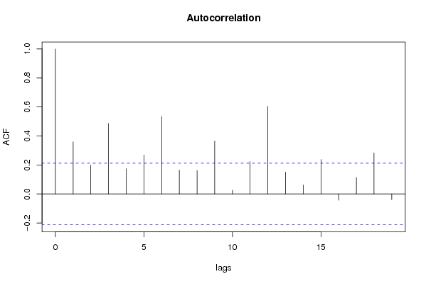
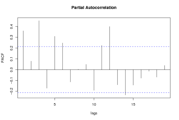
Title produced by software

(Partial) Autocorrelation Function

Date of computation

Tue, 02 Dec 2008 13:15:28 -0700

Cite this page as follows

Statistical Computations at FreeStatistics.org, Office for Research Development and Education, URL https://freestatistics.org/blog/index.php?v=date/2008/Dec/02/t12282491560hy5wqns5bcoaqf.htm/, Retrieved Sun, 19 May 2024 12:42:24 +0000

Statistical Computations at FreeStatistics.org, Office for Research Development and Education, URL https://freestatistics.org/blog/index.php?pk=28357, Retrieved Sun, 19 May 2024 12:42:24 +0000

QR Codes:

Paste this QR Code to cite your computation.

Original text written by user:

IsPrivate?

No (this computation is public)

User-defined keywords

Estimated Impact

163

Family? (F = Feedback message, R = changed R code, M = changed R Module, P = changed Parameters, D = changed Data)

F     [Univariate Data Series] [Airline data] [2007-10-18 09:58:47] [42daae401fd3def69a25014f2252b4c2]
F RMPD    [(Partial) Autocorrelation Function] [17.7.1] [2008-12-02 20:15:28] [0458bd763b171003ec052ce63099d477] [Current]
F   PD      [(Partial) Autocorrelation Function] [17.8.1] [2008-12-02 20:32:20] [1eab65e90adf64584b8e6f0da23ff414] 

Feedback Forum

2008-12-08 18:37:21 [5faab2fc6fb120339944528a32d48a04] [reply] 
Hier werd de verkeerde calculator gebruikt het was de bedoeling de Cross Correlation Function te bereken om het verband tussen de 2 variabelen duidelijk te maken.

Post a new message

Dataseries X:

Download CSV

Histogram

Boxplots

Summary of computational transaction
Raw Input	view raw input (R code)
Raw Output	view raw output of R engine
Computing time	2 seconds
R Server	'Gwilym Jenkins' @ 72.249.127.135

\begin{tabular}{lllllllll}
\hline
Summary of computational transaction \tabularnewline
Raw Input & view raw input (R code)  \tabularnewline
Raw Output & view raw output of R engine  \tabularnewline
Computing time & 2 seconds \tabularnewline
R Server & 'Gwilym Jenkins' @ 72.249.127.135 \tabularnewline
\hline
\end{tabular}
%Source: https://freestatistics.org/blog/index.php?pk=28357&T=0

[TABLE]
[ROW][C]Summary of computational transaction[/C][/ROW]
[ROW][C]Raw Input[/C][C]view raw input (R code) [/C][/ROW]
[ROW][C]Raw Output[/C][C]view raw output of R engine [/C][/ROW]
[ROW][C]Computing time[/C][C]2 seconds[/C][/ROW]
[ROW][C]R Server[/C][C]'Gwilym Jenkins' @ 72.249.127.135[/C][/ROW]
[/TABLE]
Source: https://freestatistics.org/blog/index.php?pk=28357&T=0

Globally Unique Identifier (entire table): ba.freestatistics.org/blog/index.php?pk=28357&T=0

As an alternative you can also use a QR Code:

The GUIDs for individual cells are displayed in the table below:

Summary of computational transaction
Raw Input	view raw input (R code)
Raw Output	view raw output of R engine
Computing time	2 seconds
R Server	'Gwilym Jenkins' @ 72.249.127.135

Autocorrelation Function
Time lag k	ACF(k)	T-STAT	P-value
1	0.359538	3.3148	0.000675
2	0.198261	1.8279	0.035538
3	0.486407	4.4845	1.1e-05
4	0.174528	1.6091	0.055655
5	0.269103	2.481	0.007536
6	0.533942	4.9227	2e-06
7	0.165069	1.5219	0.065878
8	0.161808	1.4918	0.069728
9	0.3648	3.3633	0.000578
10	0.02642	0.2436	0.404071
11	0.223418	2.0598	0.021238
12	0.604234	5.5708	0
13	0.151393	1.3958	0.083209
14	0.062669	0.5778	0.282469
15	0.237415	2.1889	0.015675
16	-0.043026	-0.3967	0.346298
17	0.113438	1.0458	0.149299
18	0.283185	2.6108	0.005337
19	-0.039348	-0.3628	0.358839

\begin{tabular}{lllllllll}
\hline
Autocorrelation Function \tabularnewline
Time lag k & ACF(k) & T-STAT & P-value \tabularnewline
1 & 0.359538 & 3.3148 & 0.000675 \tabularnewline
2 & 0.198261 & 1.8279 & 0.035538 \tabularnewline
3 & 0.486407 & 4.4845 & 1.1e-05 \tabularnewline
4 & 0.174528 & 1.6091 & 0.055655 \tabularnewline
5 & 0.269103 & 2.481 & 0.007536 \tabularnewline
6 & 0.533942 & 4.9227 & 2e-06 \tabularnewline
7 & 0.165069 & 1.5219 & 0.065878 \tabularnewline
8 & 0.161808 & 1.4918 & 0.069728 \tabularnewline
9 & 0.3648 & 3.3633 & 0.000578 \tabularnewline
10 & 0.02642 & 0.2436 & 0.404071 \tabularnewline
11 & 0.223418 & 2.0598 & 0.021238 \tabularnewline
12 & 0.604234 & 5.5708 & 0 \tabularnewline
13 & 0.151393 & 1.3958 & 0.083209 \tabularnewline
14 & 0.062669 & 0.5778 & 0.282469 \tabularnewline
15 & 0.237415 & 2.1889 & 0.015675 \tabularnewline
16 & -0.043026 & -0.3967 & 0.346298 \tabularnewline
17 & 0.113438 & 1.0458 & 0.149299 \tabularnewline
18 & 0.283185 & 2.6108 & 0.005337 \tabularnewline
19 & -0.039348 & -0.3628 & 0.358839 \tabularnewline
\hline
\end{tabular}
%Source: https://freestatistics.org/blog/index.php?pk=28357&T=1

[TABLE]
[ROW][C]Autocorrelation Function[/C][/ROW]
[ROW][C]Time lag k[/C][C]ACF(k)[/C][C]T-STAT[/C][C]P-value[/C][/ROW]
[ROW][C]1[/C][C]0.359538[/C][C]3.3148[/C][C]0.000675[/C][/ROW]
[ROW][C]2[/C][C]0.198261[/C][C]1.8279[/C][C]0.035538[/C][/ROW]
[ROW][C]3[/C][C]0.486407[/C][C]4.4845[/C][C]1.1e-05[/C][/ROW]
[ROW][C]4[/C][C]0.174528[/C][C]1.6091[/C][C]0.055655[/C][/ROW]
[ROW][C]5[/C][C]0.269103[/C][C]2.481[/C][C]0.007536[/C][/ROW]
[ROW][C]6[/C][C]0.533942[/C][C]4.9227[/C][C]2e-06[/C][/ROW]
[ROW][C]7[/C][C]0.165069[/C][C]1.5219[/C][C]0.065878[/C][/ROW]
[ROW][C]8[/C][C]0.161808[/C][C]1.4918[/C][C]0.069728[/C][/ROW]
[ROW][C]9[/C][C]0.3648[/C][C]3.3633[/C][C]0.000578[/C][/ROW]
[ROW][C]10[/C][C]0.02642[/C][C]0.2436[/C][C]0.404071[/C][/ROW]
[ROW][C]11[/C][C]0.223418[/C][C]2.0598[/C][C]0.021238[/C][/ROW]
[ROW][C]12[/C][C]0.604234[/C][C]5.5708[/C][C]0[/C][/ROW]
[ROW][C]13[/C][C]0.151393[/C][C]1.3958[/C][C]0.083209[/C][/ROW]
[ROW][C]14[/C][C]0.062669[/C][C]0.5778[/C][C]0.282469[/C][/ROW]
[ROW][C]15[/C][C]0.237415[/C][C]2.1889[/C][C]0.015675[/C][/ROW]
[ROW][C]16[/C][C]-0.043026[/C][C]-0.3967[/C][C]0.346298[/C][/ROW]
[ROW][C]17[/C][C]0.113438[/C][C]1.0458[/C][C]0.149299[/C][/ROW]
[ROW][C]18[/C][C]0.283185[/C][C]2.6108[/C][C]0.005337[/C][/ROW]
[ROW][C]19[/C][C]-0.039348[/C][C]-0.3628[/C][C]0.358839[/C][/ROW]
[/TABLE]
Source: https://freestatistics.org/blog/index.php?pk=28357&T=1

Globally Unique Identifier (entire table): ba.freestatistics.org/blog/index.php?pk=28357&T=1

As an alternative you can also use a QR Code:

The GUIDs for individual cells are displayed in the table below:

Autocorrelation Function
Time lag k	ACF(k)	T-STAT	P-value
1	0.359538	3.3148	0.000675
2	0.198261	1.8279	0.035538
3	0.486407	4.4845	1.1e-05
4	0.174528	1.6091	0.055655
5	0.269103	2.481	0.007536
6	0.533942	4.9227	2e-06
7	0.165069	1.5219	0.065878
8	0.161808	1.4918	0.069728
9	0.3648	3.3633	0.000578
10	0.02642	0.2436	0.404071
11	0.223418	2.0598	0.021238
12	0.604234	5.5708	0
13	0.151393	1.3958	0.083209
14	0.062669	0.5778	0.282469
15	0.237415	2.1889	0.015675
16	-0.043026	-0.3967	0.346298
17	0.113438	1.0458	0.149299
18	0.283185	2.6108	0.005337
19	-0.039348	-0.3628	0.358839

Partial Autocorrelation Function
Time lag k	PACF(k)	T-STAT	P-value
1	0.359538	3.3148	0.000675
2	0.079236	0.7305	0.233541
3	0.453369	4.1799	3.5e-05
4	-0.171629	-1.5823	0.058643
5	0.309026	2.8491	0.002749
6	0.247102	2.2782	0.012613
7	-0.113711	-1.0484	0.148721
8	0.004331	0.0399	0.484121
9	0.049101	0.4527	0.325962
10	-0.191573	-1.7662	0.040475
11	0.224567	2.0704	0.020724
12	0.399173	3.6802	0.000204
13	-0.140109	-1.2917	0.099975
14	-0.234495	-2.1619	0.016717
15	-0.14282	-1.3167	0.095734
16	-0.078857	-0.727	0.234604
17	-0.014838	-0.1368	0.445758
18	-0.069026	-0.6364	0.263118
19	0.039188	0.3613	0.359387

\begin{tabular}{lllllllll}
\hline
Partial Autocorrelation Function \tabularnewline
Time lag k & PACF(k) & T-STAT & P-value \tabularnewline
1 & 0.359538 & 3.3148 & 0.000675 \tabularnewline
2 & 0.079236 & 0.7305 & 0.233541 \tabularnewline
3 & 0.453369 & 4.1799 & 3.5e-05 \tabularnewline
4 & -0.171629 & -1.5823 & 0.058643 \tabularnewline
5 & 0.309026 & 2.8491 & 0.002749 \tabularnewline
6 & 0.247102 & 2.2782 & 0.012613 \tabularnewline
7 & -0.113711 & -1.0484 & 0.148721 \tabularnewline
8 & 0.004331 & 0.0399 & 0.484121 \tabularnewline
9 & 0.049101 & 0.4527 & 0.325962 \tabularnewline
10 & -0.191573 & -1.7662 & 0.040475 \tabularnewline
11 & 0.224567 & 2.0704 & 0.020724 \tabularnewline
12 & 0.399173 & 3.6802 & 0.000204 \tabularnewline
13 & -0.140109 & -1.2917 & 0.099975 \tabularnewline
14 & -0.234495 & -2.1619 & 0.016717 \tabularnewline
15 & -0.14282 & -1.3167 & 0.095734 \tabularnewline
16 & -0.078857 & -0.727 & 0.234604 \tabularnewline
17 & -0.014838 & -0.1368 & 0.445758 \tabularnewline
18 & -0.069026 & -0.6364 & 0.263118 \tabularnewline
19 & 0.039188 & 0.3613 & 0.359387 \tabularnewline
\hline
\end{tabular}
%Source: https://freestatistics.org/blog/index.php?pk=28357&T=2

[TABLE]
[ROW][C]Partial Autocorrelation Function[/C][/ROW]
[ROW][C]Time lag k[/C][C]PACF(k)[/C][C]T-STAT[/C][C]P-value[/C][/ROW]
[ROW][C]1[/C][C]0.359538[/C][C]3.3148[/C][C]0.000675[/C][/ROW]
[ROW][C]2[/C][C]0.079236[/C][C]0.7305[/C][C]0.233541[/C][/ROW]
[ROW][C]3[/C][C]0.453369[/C][C]4.1799[/C][C]3.5e-05[/C][/ROW]
[ROW][C]4[/C][C]-0.171629[/C][C]-1.5823[/C][C]0.058643[/C][/ROW]
[ROW][C]5[/C][C]0.309026[/C][C]2.8491[/C][C]0.002749[/C][/ROW]
[ROW][C]6[/C][C]0.247102[/C][C]2.2782[/C][C]0.012613[/C][/ROW]
[ROW][C]7[/C][C]-0.113711[/C][C]-1.0484[/C][C]0.148721[/C][/ROW]
[ROW][C]8[/C][C]0.004331[/C][C]0.0399[/C][C]0.484121[/C][/ROW]
[ROW][C]9[/C][C]0.049101[/C][C]0.4527[/C][C]0.325962[/C][/ROW]
[ROW][C]10[/C][C]-0.191573[/C][C]-1.7662[/C][C]0.040475[/C][/ROW]
[ROW][C]11[/C][C]0.224567[/C][C]2.0704[/C][C]0.020724[/C][/ROW]
[ROW][C]12[/C][C]0.399173[/C][C]3.6802[/C][C]0.000204[/C][/ROW]
[ROW][C]13[/C][C]-0.140109[/C][C]-1.2917[/C][C]0.099975[/C][/ROW]
[ROW][C]14[/C][C]-0.234495[/C][C]-2.1619[/C][C]0.016717[/C][/ROW]
[ROW][C]15[/C][C]-0.14282[/C][C]-1.3167[/C][C]0.095734[/C][/ROW]
[ROW][C]16[/C][C]-0.078857[/C][C]-0.727[/C][C]0.234604[/C][/ROW]
[ROW][C]17[/C][C]-0.014838[/C][C]-0.1368[/C][C]0.445758[/C][/ROW]
[ROW][C]18[/C][C]-0.069026[/C][C]-0.6364[/C][C]0.263118[/C][/ROW]
[ROW][C]19[/C][C]0.039188[/C][C]0.3613[/C][C]0.359387[/C][/ROW]
[/TABLE]
Source: https://freestatistics.org/blog/index.php?pk=28357&T=2

Globally Unique Identifier (entire table): ba.freestatistics.org/blog/index.php?pk=28357&T=2

As an alternative you can also use a QR Code:

The GUIDs for individual cells are displayed in the table below:

Partial Autocorrelation Function
Time lag k	PACF(k)	T-STAT	P-value
1	0.359538	3.3148	0.000675
2	0.079236	0.7305	0.233541
3	0.453369	4.1799	3.5e-05
4	-0.171629	-1.5823	0.058643
5	0.309026	2.8491	0.002749
6	0.247102	2.2782	0.012613
7	-0.113711	-1.0484	0.148721
8	0.004331	0.0399	0.484121
9	0.049101	0.4527	0.325962
10	-0.191573	-1.7662	0.040475
11	0.224567	2.0704	0.020724
12	0.399173	3.6802	0.000204
13	-0.140109	-1.2917	0.099975
14	-0.234495	-2.1619	0.016717
15	-0.14282	-1.3167	0.095734
16	-0.078857	-0.727	0.234604
17	-0.014838	-0.1368	0.445758
18	-0.069026	-0.6364	0.263118
19	0.039188	0.3613	0.359387

Figure 1

PNG link

Postscript link

PDF link

Figure 2

PNG link

Postscript link

PDF link

Parameters (Session):

par1 = Default ; par2 = 1 ; par3 = 0 ; par4 = 0 ; par5 = 12 ;

Parameters (R input):

par1 = Default ; par2 = 1 ; par3 = 0 ; par4 = 0 ; par5 = 12 ;

R code (references can be found in the software module):

if (par1 == 'Default') {
par1 = 10*log10(length(x))
} else {
par1 <- as.numeric(par1)
}
par2 <- as.numeric(par2)
par3 <- as.numeric(par3)
par4 <- as.numeric(par4)
par5 <- as.numeric(par5)
if (par2 == 0) {
x <- log(x)
} else {
x <- (x ^ par2 - 1) / par2
}
if (par3 > 0) x <- diff(x,lag=1,difference=par3)
if (par4 > 0) x <- diff(x,lag=par5,difference=par4)
bitmap(file='pic1.png')
racf <- acf(x,par1,main='Autocorrelation',xlab='lags',ylab='ACF')
dev.off()
bitmap(file='pic2.png')
rpacf <- pacf(x,par1,main='Partial Autocorrelation',xlab='lags',ylab='PACF')
dev.off()
(myacf <- c(racf$acf))
(mypacf <- c(rpacf$acf))
lengthx <- length(x)
sqrtn <- sqrt(lengthx)
load(file='createtable')
a<-table.start()
a<-table.row.start(a)
a<-table.element(a,'Autocorrelation Function',4,TRUE)
a<-table.row.end(a)
a<-table.row.start(a)
a<-table.element(a,'Time lag k',header=TRUE)
a<-table.element(a,hyperlink('basics.htm','ACF(k)','click here for more information about the Autocorrelation Function'),header=TRUE)
a<-table.element(a,'T-STAT',header=TRUE)
a<-table.element(a,'P-value',header=TRUE)
a<-table.row.end(a)
for (i in 2:(par1+1)) {
a<-table.row.start(a)
a<-table.element(a,i-1,header=TRUE)
a<-table.element(a,round(myacf[i],6))
mytstat <- myacf[i]*sqrtn
a<-table.element(a,round(mytstat,4))
a<-table.element(a,round(1-pt(abs(mytstat),lengthx),6))
a<-table.row.end(a)
}
a<-table.end(a)
table.save(a,file='mytable.tab')
a<-table.start()
a<-table.row.start(a)
a<-table.element(a,'Partial Autocorrelation Function',4,TRUE)
a<-table.row.end(a)
a<-table.row.start(a)
a<-table.element(a,'Time lag k',header=TRUE)
a<-table.element(a,hyperlink('basics.htm','PACF(k)','click here for more information about the Partial Autocorrelation Function'),header=TRUE)
a<-table.element(a,'T-STAT',header=TRUE)
a<-table.element(a,'P-value',header=TRUE)
a<-table.row.end(a)
for (i in 1:par1) {
a<-table.row.start(a)
a<-table.element(a,i,header=TRUE)
a<-table.element(a,round(mypacf[i],6))
mytstat <- mypacf[i]*sqrtn
a<-table.element(a,round(mytstat,4))
a<-table.element(a,round(1-pt(abs(mytstat),lengthx),6))
a<-table.row.end(a)
}
a<-table.end(a)
table.save(a,file='mytable1.tab')

Free Statistics

Description of Statistical Computation

Tree of Dependent Computations

Dataset

Tables (Output of Computation)

Figures (Output of Computation)

Input Parameters & R Code