Repository of Reproducible Computations

Free Statistics

of Irreproducible Research!

Author's title

Author

*Unverified author*

R Software Module

rwasp_autocorrelation.wasp

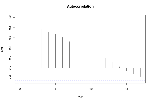
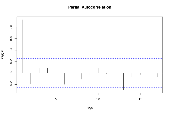
Title produced by software

(Partial) Autocorrelation Function

Date of computation

Tue, 02 Dec 2008 13:08:00 -0700

Cite this page as follows

Statistical Computations at FreeStatistics.org, Office for Research Development and Education, URL https://freestatistics.org/blog/index.php?v=date/2008/Dec/02/t12282485827yip4leqq0gmvpl.htm/, Retrieved Sun, 19 May 2024 10:46:35 +0000

Statistical Computations at FreeStatistics.org, Office for Research Development and Education, URL https://freestatistics.org/blog/index.php?pk=28330, Retrieved Sun, 19 May 2024 10:46:35 +0000

QR Codes:

Paste this QR Code to cite your computation.

Original text written by user:

IsPrivate?

No (this computation is public)

User-defined keywords

Estimated Impact

140

Family? (F = Feedback message, R = changed R code, M = changed R Module, P = changed Parameters, D = changed Data)

F       [(Partial) Autocorrelation Function] [autocorrelation] [2008-12-02 20:08:00] [72e979bcc364082694890d2eccc1a66f] [Current]
-   PD    [(Partial) Autocorrelation Function] [autocorrelation] [2008-12-02 20:10:31] [c94d7012e41b73cfa20d93e879679ede] 
-   PD      [(Partial) Autocorrelation Function] [autocorrelation] [2008-12-02 20:13:09] [c94d7012e41b73cfa20d93e879679ede] 
-   PD        [(Partial) Autocorrelation Function] [autocorrelation] [2008-12-02 20:15:11] [c94d7012e41b73cfa20d93e879679ede] 
F RMPD        [Cross Correlation Function] [cross correlation] [2008-12-02 20:19:09] [c94d7012e41b73cfa20d93e879679ede] 

Feedback Forum

2008-12-04 09:13:44 [Julie Govaerts] [reply] 
je kan ook gebruik maken van de VRM of de spectrale analyse
2008-12-04 14:07:12 [72e979bcc364082694890d2eccc1a66f] [reply] 
Hier werd gebruik gemaakt van de verkeerde software. Om de lambda te berekenen gebruiken we de standard deviation mean plot. Daaruit kan je dan makkelijk de lambda aflezen. 
Om d en D te bepalen maken we gebruik van de variance reduction matrix. Hier ga je dan op zoek naar de kleinste variantie en daarnaast vind je dan de gepaste waarden voor d en D.

Post a new message

Dataseries X:

Download CSV

Histogram

Boxplots

Summary of computational transaction
Raw Input	view raw input (R code)
Raw Output	view raw output of R engine
Computing time	1 seconds
R Server	'Gwilym Jenkins' @ 72.249.127.135

\begin{tabular}{lllllllll}
\hline
Summary of computational transaction \tabularnewline
Raw Input & view raw input (R code)  \tabularnewline
Raw Output & view raw output of R engine  \tabularnewline
Computing time & 1 seconds \tabularnewline
R Server & 'Gwilym Jenkins' @ 72.249.127.135 \tabularnewline
\hline
\end{tabular}
%Source: https://freestatistics.org/blog/index.php?pk=28330&T=0

[TABLE]
[ROW][C]Summary of computational transaction[/C][/ROW]
[ROW][C]Raw Input[/C][C]view raw input (R code) [/C][/ROW]
[ROW][C]Raw Output[/C][C]view raw output of R engine [/C][/ROW]
[ROW][C]Computing time[/C][C]1 seconds[/C][/ROW]
[ROW][C]R Server[/C][C]'Gwilym Jenkins' @ 72.249.127.135[/C][/ROW]
[/TABLE]
Source: https://freestatistics.org/blog/index.php?pk=28330&T=0

Globally Unique Identifier (entire table): ba.freestatistics.org/blog/index.php?pk=28330&T=0

As an alternative you can also use a QR Code:

The GUIDs for individual cells are displayed in the table below:

Summary of computational transaction
Raw Input	view raw input (R code)
Raw Output	view raw output of R engine
Computing time	1 seconds
R Server	'Gwilym Jenkins' @ 72.249.127.135

Autocorrelation Function
Time lag k	ACF(k)	T-STAT	P-value
1	0.93222	7.2209	0
2	0.843594	6.5344	0
3	0.768274	5.951	0
4	0.714199	5.5322	0
5	0.671747	5.2033	1e-06
6	0.607631	4.7067	8e-06
7	0.524814	4.0652	7.1e-05
8	0.432474	3.3499	0.000701
9	0.34791	2.6949	0.00456
10	0.29002	2.2465	0.014183
11	0.242708	1.88	0.032482
12	0.200509	1.5531	0.062825
13	0.120801	0.9357	0.176584
14	0.025954	0.201	0.420675
15	-0.055246	-0.4279	0.335117
16	-0.119842	-0.9283	0.178488
17	-0.171306	-1.3269	0.09478

\begin{tabular}{lllllllll}
\hline
Autocorrelation Function \tabularnewline
Time lag k & ACF(k) & T-STAT & P-value \tabularnewline
1 & 0.93222 & 7.2209 & 0 \tabularnewline
2 & 0.843594 & 6.5344 & 0 \tabularnewline
3 & 0.768274 & 5.951 & 0 \tabularnewline
4 & 0.714199 & 5.5322 & 0 \tabularnewline
5 & 0.671747 & 5.2033 & 1e-06 \tabularnewline
6 & 0.607631 & 4.7067 & 8e-06 \tabularnewline
7 & 0.524814 & 4.0652 & 7.1e-05 \tabularnewline
8 & 0.432474 & 3.3499 & 0.000701 \tabularnewline
9 & 0.34791 & 2.6949 & 0.00456 \tabularnewline
10 & 0.29002 & 2.2465 & 0.014183 \tabularnewline
11 & 0.242708 & 1.88 & 0.032482 \tabularnewline
12 & 0.200509 & 1.5531 & 0.062825 \tabularnewline
13 & 0.120801 & 0.9357 & 0.176584 \tabularnewline
14 & 0.025954 & 0.201 & 0.420675 \tabularnewline
15 & -0.055246 & -0.4279 & 0.335117 \tabularnewline
16 & -0.119842 & -0.9283 & 0.178488 \tabularnewline
17 & -0.171306 & -1.3269 & 0.09478 \tabularnewline
\hline
\end{tabular}
%Source: https://freestatistics.org/blog/index.php?pk=28330&T=1

[TABLE]
[ROW][C]Autocorrelation Function[/C][/ROW]
[ROW][C]Time lag k[/C][C]ACF(k)[/C][C]T-STAT[/C][C]P-value[/C][/ROW]
[ROW][C]1[/C][C]0.93222[/C][C]7.2209[/C][C]0[/C][/ROW]
[ROW][C]2[/C][C]0.843594[/C][C]6.5344[/C][C]0[/C][/ROW]
[ROW][C]3[/C][C]0.768274[/C][C]5.951[/C][C]0[/C][/ROW]
[ROW][C]4[/C][C]0.714199[/C][C]5.5322[/C][C]0[/C][/ROW]
[ROW][C]5[/C][C]0.671747[/C][C]5.2033[/C][C]1e-06[/C][/ROW]
[ROW][C]6[/C][C]0.607631[/C][C]4.7067[/C][C]8e-06[/C][/ROW]
[ROW][C]7[/C][C]0.524814[/C][C]4.0652[/C][C]7.1e-05[/C][/ROW]
[ROW][C]8[/C][C]0.432474[/C][C]3.3499[/C][C]0.000701[/C][/ROW]
[ROW][C]9[/C][C]0.34791[/C][C]2.6949[/C][C]0.00456[/C][/ROW]
[ROW][C]10[/C][C]0.29002[/C][C]2.2465[/C][C]0.014183[/C][/ROW]
[ROW][C]11[/C][C]0.242708[/C][C]1.88[/C][C]0.032482[/C][/ROW]
[ROW][C]12[/C][C]0.200509[/C][C]1.5531[/C][C]0.062825[/C][/ROW]
[ROW][C]13[/C][C]0.120801[/C][C]0.9357[/C][C]0.176584[/C][/ROW]
[ROW][C]14[/C][C]0.025954[/C][C]0.201[/C][C]0.420675[/C][/ROW]
[ROW][C]15[/C][C]-0.055246[/C][C]-0.4279[/C][C]0.335117[/C][/ROW]
[ROW][C]16[/C][C]-0.119842[/C][C]-0.9283[/C][C]0.178488[/C][/ROW]
[ROW][C]17[/C][C]-0.171306[/C][C]-1.3269[/C][C]0.09478[/C][/ROW]
[/TABLE]
Source: https://freestatistics.org/blog/index.php?pk=28330&T=1

Globally Unique Identifier (entire table): ba.freestatistics.org/blog/index.php?pk=28330&T=1

As an alternative you can also use a QR Code:

The GUIDs for individual cells are displayed in the table below:

Autocorrelation Function
Time lag k	ACF(k)	T-STAT	P-value
1	0.93222	7.2209	0
2	0.843594	6.5344	0
3	0.768274	5.951	0
4	0.714199	5.5322	0
5	0.671747	5.2033	1e-06
6	0.607631	4.7067	8e-06
7	0.524814	4.0652	7.1e-05
8	0.432474	3.3499	0.000701
9	0.34791	2.6949	0.00456
10	0.29002	2.2465	0.014183
11	0.242708	1.88	0.032482
12	0.200509	1.5531	0.062825
13	0.120801	0.9357	0.176584
14	0.025954	0.201	0.420675
15	-0.055246	-0.4279	0.335117
16	-0.119842	-0.9283	0.178488
17	-0.171306	-1.3269	0.09478

Partial Autocorrelation Function
Time lag k	PACF(k)	T-STAT	P-value
1	0.93222	7.2209	0
2	-0.19426	-1.5047	0.06882
3	0.080798	0.6259	0.26689
4	0.089856	0.696	0.244551
5	0.024018	0.186	0.426519
6	-0.196842	-1.5247	0.06629
7	-0.107867	-0.8355	0.203365
8	-0.108355	-0.8393	0.202313
9	-0.032342	-0.2505	0.401521
10	0.087219	0.6756	0.250946
11	-0.008696	-0.0674	0.473261
12	0.042312	0.3277	0.372123
13	-0.30004	-2.3241	0.011762
14	-0.07353	-0.5696	0.28555
15	-0.025339	-0.1963	0.422528
16	-0.057962	-0.449	0.327534
17	-0.063397	-0.4911	0.312584

\begin{tabular}{lllllllll}
\hline
Partial Autocorrelation Function \tabularnewline
Time lag k & PACF(k) & T-STAT & P-value \tabularnewline
1 & 0.93222 & 7.2209 & 0 \tabularnewline
2 & -0.19426 & -1.5047 & 0.06882 \tabularnewline
3 & 0.080798 & 0.6259 & 0.26689 \tabularnewline
4 & 0.089856 & 0.696 & 0.244551 \tabularnewline
5 & 0.024018 & 0.186 & 0.426519 \tabularnewline
6 & -0.196842 & -1.5247 & 0.06629 \tabularnewline
7 & -0.107867 & -0.8355 & 0.203365 \tabularnewline
8 & -0.108355 & -0.8393 & 0.202313 \tabularnewline
9 & -0.032342 & -0.2505 & 0.401521 \tabularnewline
10 & 0.087219 & 0.6756 & 0.250946 \tabularnewline
11 & -0.008696 & -0.0674 & 0.473261 \tabularnewline
12 & 0.042312 & 0.3277 & 0.372123 \tabularnewline
13 & -0.30004 & -2.3241 & 0.011762 \tabularnewline
14 & -0.07353 & -0.5696 & 0.28555 \tabularnewline
15 & -0.025339 & -0.1963 & 0.422528 \tabularnewline
16 & -0.057962 & -0.449 & 0.327534 \tabularnewline
17 & -0.063397 & -0.4911 & 0.312584 \tabularnewline
\hline
\end{tabular}
%Source: https://freestatistics.org/blog/index.php?pk=28330&T=2

[TABLE]
[ROW][C]Partial Autocorrelation Function[/C][/ROW]
[ROW][C]Time lag k[/C][C]PACF(k)[/C][C]T-STAT[/C][C]P-value[/C][/ROW]
[ROW][C]1[/C][C]0.93222[/C][C]7.2209[/C][C]0[/C][/ROW]
[ROW][C]2[/C][C]-0.19426[/C][C]-1.5047[/C][C]0.06882[/C][/ROW]
[ROW][C]3[/C][C]0.080798[/C][C]0.6259[/C][C]0.26689[/C][/ROW]
[ROW][C]4[/C][C]0.089856[/C][C]0.696[/C][C]0.244551[/C][/ROW]
[ROW][C]5[/C][C]0.024018[/C][C]0.186[/C][C]0.426519[/C][/ROW]
[ROW][C]6[/C][C]-0.196842[/C][C]-1.5247[/C][C]0.06629[/C][/ROW]
[ROW][C]7[/C][C]-0.107867[/C][C]-0.8355[/C][C]0.203365[/C][/ROW]
[ROW][C]8[/C][C]-0.108355[/C][C]-0.8393[/C][C]0.202313[/C][/ROW]
[ROW][C]9[/C][C]-0.032342[/C][C]-0.2505[/C][C]0.401521[/C][/ROW]
[ROW][C]10[/C][C]0.087219[/C][C]0.6756[/C][C]0.250946[/C][/ROW]
[ROW][C]11[/C][C]-0.008696[/C][C]-0.0674[/C][C]0.473261[/C][/ROW]
[ROW][C]12[/C][C]0.042312[/C][C]0.3277[/C][C]0.372123[/C][/ROW]
[ROW][C]13[/C][C]-0.30004[/C][C]-2.3241[/C][C]0.011762[/C][/ROW]
[ROW][C]14[/C][C]-0.07353[/C][C]-0.5696[/C][C]0.28555[/C][/ROW]
[ROW][C]15[/C][C]-0.025339[/C][C]-0.1963[/C][C]0.422528[/C][/ROW]
[ROW][C]16[/C][C]-0.057962[/C][C]-0.449[/C][C]0.327534[/C][/ROW]
[ROW][C]17[/C][C]-0.063397[/C][C]-0.4911[/C][C]0.312584[/C][/ROW]
[/TABLE]
Source: https://freestatistics.org/blog/index.php?pk=28330&T=2

Globally Unique Identifier (entire table): ba.freestatistics.org/blog/index.php?pk=28330&T=2

As an alternative you can also use a QR Code:

The GUIDs for individual cells are displayed in the table below:

Partial Autocorrelation Function
Time lag k	PACF(k)	T-STAT	P-value
1	0.93222	7.2209	0
2	-0.19426	-1.5047	0.06882
3	0.080798	0.6259	0.26689
4	0.089856	0.696	0.244551
5	0.024018	0.186	0.426519
6	-0.196842	-1.5247	0.06629
7	-0.107867	-0.8355	0.203365
8	-0.108355	-0.8393	0.202313
9	-0.032342	-0.2505	0.401521
10	0.087219	0.6756	0.250946
11	-0.008696	-0.0674	0.473261
12	0.042312	0.3277	0.372123
13	-0.30004	-2.3241	0.011762
14	-0.07353	-0.5696	0.28555
15	-0.025339	-0.1963	0.422528
16	-0.057962	-0.449	0.327534
17	-0.063397	-0.4911	0.312584

Figure 1

PNG link

Postscript link

PDF link

Figure 2

PNG link

Postscript link

PDF link

Parameters (Session):

par1 = Default ; par2 = 1 ; par3 = 0 ; par4 = 0 ; par5 = 12 ;

Parameters (R input):

par1 = Default ; par2 = 1 ; par3 = 0 ; par4 = 0 ; par5 = 12 ;

R code (references can be found in the software module):

if (par1 == 'Default') {
par1 = 10*log10(length(x))
} else {
par1 <- as.numeric(par1)
}
par2 <- as.numeric(par2)
par3 <- as.numeric(par3)
par4 <- as.numeric(par4)
par5 <- as.numeric(par5)
if (par2 == 0) {
x <- log(x)
} else {
x <- (x ^ par2 - 1) / par2
}
if (par3 > 0) x <- diff(x,lag=1,difference=par3)
if (par4 > 0) x <- diff(x,lag=par5,difference=par4)
bitmap(file='pic1.png')
racf <- acf(x,par1,main='Autocorrelation',xlab='lags',ylab='ACF')
dev.off()
bitmap(file='pic2.png')
rpacf <- pacf(x,par1,main='Partial Autocorrelation',xlab='lags',ylab='PACF')
dev.off()
(myacf <- c(racf$acf))
(mypacf <- c(rpacf$acf))
lengthx <- length(x)
sqrtn <- sqrt(lengthx)
load(file='createtable')
a<-table.start()
a<-table.row.start(a)
a<-table.element(a,'Autocorrelation Function',4,TRUE)
a<-table.row.end(a)
a<-table.row.start(a)
a<-table.element(a,'Time lag k',header=TRUE)
a<-table.element(a,hyperlink('basics.htm','ACF(k)','click here for more information about the Autocorrelation Function'),header=TRUE)
a<-table.element(a,'T-STAT',header=TRUE)
a<-table.element(a,'P-value',header=TRUE)
a<-table.row.end(a)
for (i in 2:(par1+1)) {
a<-table.row.start(a)
a<-table.element(a,i-1,header=TRUE)
a<-table.element(a,round(myacf[i],6))
mytstat <- myacf[i]*sqrtn
a<-table.element(a,round(mytstat,4))
a<-table.element(a,round(1-pt(abs(mytstat),lengthx),6))
a<-table.row.end(a)
}
a<-table.end(a)
table.save(a,file='mytable.tab')
a<-table.start()
a<-table.row.start(a)
a<-table.element(a,'Partial Autocorrelation Function',4,TRUE)
a<-table.row.end(a)
a<-table.row.start(a)
a<-table.element(a,'Time lag k',header=TRUE)
a<-table.element(a,hyperlink('basics.htm','PACF(k)','click here for more information about the Partial Autocorrelation Function'),header=TRUE)
a<-table.element(a,'T-STAT',header=TRUE)
a<-table.element(a,'P-value',header=TRUE)
a<-table.row.end(a)
for (i in 1:par1) {
a<-table.row.start(a)
a<-table.element(a,i,header=TRUE)
a<-table.element(a,round(mypacf[i],6))
mytstat <- mypacf[i]*sqrtn
a<-table.element(a,round(mytstat,4))
a<-table.element(a,round(1-pt(abs(mytstat),lengthx),6))
a<-table.row.end(a)
}
a<-table.end(a)
table.save(a,file='mytable1.tab')

Free Statistics

Description of Statistical Computation

Tree of Dependent Computations

Dataset

Tables (Output of Computation)

Figures (Output of Computation)

Input Parameters & R Code