Free Statistics
of Irreproducible Research!
Description of Statistical Computation | |||||||||||||||||||||||||||||||||
|---|---|---|---|---|---|---|---|---|---|---|---|---|---|---|---|---|---|---|---|---|---|---|---|---|---|---|---|---|---|---|---|---|---|
| Author's title | sven van roy - tweede zittijd - oefening 2.2 - eigen reeks - dichtheidsgraf... | ||||||||||||||||||||||||||||||||
| Author | *Unverified author* | ||||||||||||||||||||||||||||||||
| R Software Module | rwasp_density.wasp | ||||||||||||||||||||||||||||||||
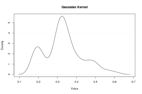
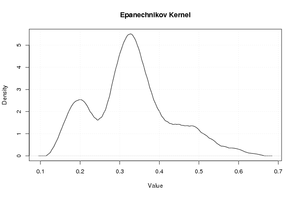
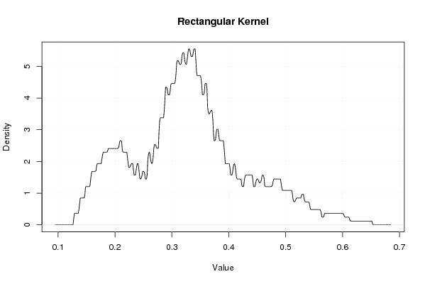
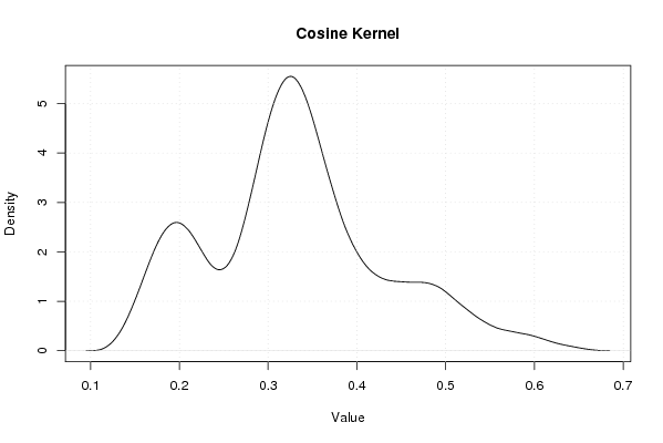
| Title produced by software | Kernel Density Estimation | ||||||||||||||||||||||||||||||||
| Date of computation | Mon, 11 Aug 2008 08:09:24 -0600 | ||||||||||||||||||||||||||||||||
| Cite this page as follows | Statistical Computations at FreeStatistics.org, Office for Research Development and Education, URL https://freestatistics.org/blog/index.php?v=date/2008/Aug/11/t1218463851uuv60h4cvez5235.htm/, Retrieved Tue, 14 May 2024 16:16:22 +0000 | ||||||||||||||||||||||||||||||||
| Statistical Computations at FreeStatistics.org, Office for Research Development and Education, URL https://freestatistics.org/blog/index.php?pk=13948, Retrieved Tue, 14 May 2024 16:16:22 +0000 | |||||||||||||||||||||||||||||||||
| QR Codes: | |||||||||||||||||||||||||||||||||
|
| |||||||||||||||||||||||||||||||||
| Original text written by user: | |||||||||||||||||||||||||||||||||
| IsPrivate? | No (this computation is public) | ||||||||||||||||||||||||||||||||
| User-defined keywords | |||||||||||||||||||||||||||||||||
| Estimated Impact | 255 | ||||||||||||||||||||||||||||||||
Tree of Dependent Computations | |||||||||||||||||||||||||||||||||
| Family? (F = Feedback message, R = changed R code, M = changed R Module, P = changed Parameters, D = changed Data) | |||||||||||||||||||||||||||||||||
| - [Histogram] [sven van roy - tw...] [2008-07-24 20:25:01] [f85cc8f00ef4b762f0a6fdfddc793773] - RMPD [Kernel Density Estimation] [sven van roy - tw...] [2008-08-11 14:09:24] [9ed44c8445a965e8d6beecda46dd06a5] [Current] | |||||||||||||||||||||||||||||||||
| Feedback Forum | |||||||||||||||||||||||||||||||||
Post a new message | |||||||||||||||||||||||||||||||||
Dataset | |||||||||||||||||||||||||||||||||
| Dataseries X: | |||||||||||||||||||||||||||||||||
0,22 0,22 0,2 0,21 0,21 0,19 0,19 0,18 0,18 0,19 0,18 0,17 0,17 0,17 0,18 0,2 0,2 0,2 0,22 0,23 0,25 0,25 0,27 0,29 0,3 0,31 0,33 0,31 0,33 0,33 0,35 0,37 0,47 0,45 0,45 0,4 0,34 0,35 0,34 0,35 0,36 0,37 0,36 0,35 0,36 0,33 0,3 0,28 0,28 0,28 0,3 0,32 0,32 0,3 0,3 0,31 0,33 0,34 0,31 0,33 0,35 0,38 0,4 0,32 0,29 0,3 0,3 0,32 0,32 0,32 0,32 0,32 0,33 0,31 0,33 0,35 0,37 0,37 0,38 0,42 0,42 0,49 0,45 0,41 0,4 0,42 0,47 0,49 0,47 0,52 0,56 0,57 0,61 0,52 0,5 0,5 | |||||||||||||||||||||||||||||||||
Tables (Output of Computation) | |||||||||||||||||||||||||||||||||
| |||||||||||||||||||||||||||||||||
Figures (Output of Computation) | |||||||||||||||||||||||||||||||||
Input Parameters & R Code | |||||||||||||||||||||||||||||||||
| Parameters (Session): | |||||||||||||||||||||||||||||||||
| Parameters (R input): | |||||||||||||||||||||||||||||||||
| R code (references can be found in the software module): | |||||||||||||||||||||||||||||||||
bitmap(file='density1.png') | |||||||||||||||||||||||||||||||||