Free Statistics
of Irreproducible Research!
Description of Statistical Computation | |||||||||||||||||||||
|---|---|---|---|---|---|---|---|---|---|---|---|---|---|---|---|---|---|---|---|---|---|
| Author's title | |||||||||||||||||||||
| Author | *Unverified author* | ||||||||||||||||||||
| R Software Module | rwasp_meanplot.wasp | ||||||||||||||||||||
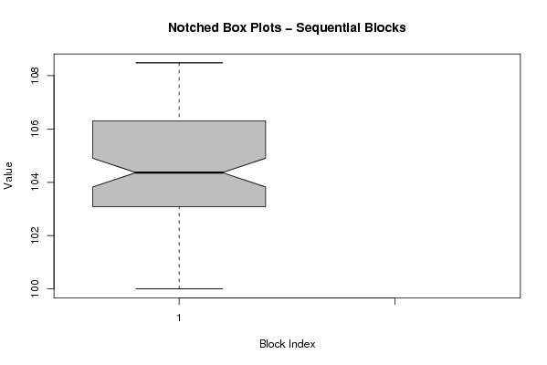
| Title produced by software | Mean Plot | ||||||||||||||||||||
| Date of computation | Mon, 29 Oct 2007 11:35:53 -0700 | ||||||||||||||||||||
| Cite this page as follows | Statistical Computations at FreeStatistics.org, Office for Research Development and Education, URL https://freestatistics.org/blog/index.php?v=date/2007/Oct/29/me978ra071xcwpt1193682963.htm/, Retrieved Sun, 05 May 2024 20:27:08 +0000 | ||||||||||||||||||||
| Statistical Computations at FreeStatistics.org, Office for Research Development and Education, URL https://freestatistics.org/blog/index.php?pk=2129, Retrieved Sun, 05 May 2024 20:27:08 +0000 | |||||||||||||||||||||
| QR Codes: | |||||||||||||||||||||
|
| |||||||||||||||||||||
| Original text written by user: | |||||||||||||||||||||
| IsPrivate? | No (this computation is public) | ||||||||||||||||||||
| User-defined keywords | |||||||||||||||||||||
| Estimated Impact | 185 | ||||||||||||||||||||
Tree of Dependent Computations | |||||||||||||||||||||
| Family? (F = Feedback message, R = changed R code, M = changed R Module, P = changed Parameters, D = changed Data) | |||||||||||||||||||||
| - [Mean Plot] [] [2007-10-29 18:35:53] [6552dbdb87730106b738e8affc0d90fa] [Current] | |||||||||||||||||||||
| Feedback Forum | |||||||||||||||||||||
Post a new message | |||||||||||||||||||||
Dataset | |||||||||||||||||||||
| Dataseries X: | |||||||||||||||||||||
100,00 100,33 100,50 100,68 100,49 100,17 100,13 100,50 101,19 101,25 101,18 101,25 101,00 101,22 101,46 102,05 102,62 102,90 103,10 103,51 103,45 103,50 104,08 104,48 104,75 104,70 104,33 104,11 104,43 104,85 105,11 104,68 105,16 104,71 104,51 104,59 104,40 103,83 103,96 103,71 103,37 103,48 103,15 102,91 103,10 103,03 103,02 103,02 103,31 103,08 103,53 103,68 103,54 103,72 103,94 103,92 104,28 105,03 105,43 105,80 106,03 106,05 106,00 106,50 106,78 106,55 106,46 106,51 106,36 106,42 106,51 106,29 106,01 106,03 106,31 106,19 106,52 106,71 107,00 107,02 107,31 107,23 107,19 107,36 107,51 107,86 108,34 108,48 108,22 108,04 | |||||||||||||||||||||
Tables (Output of Computation) | |||||||||||||||||||||
| |||||||||||||||||||||
Figures (Output of Computation) | |||||||||||||||||||||
Input Parameters & R Code | |||||||||||||||||||||
| Parameters (Session): | |||||||||||||||||||||
| par1 = 90 ; | |||||||||||||||||||||
| Parameters (R input): | |||||||||||||||||||||
| par1 = 90 ; | |||||||||||||||||||||
| R code (references can be found in the software module): | |||||||||||||||||||||
par1 <- as.numeric(par1) | |||||||||||||||||||||