Free Statistics
of Irreproducible Research!
Description of Statistical Computation | |||||||||||||||||||||
|---|---|---|---|---|---|---|---|---|---|---|---|---|---|---|---|---|---|---|---|---|---|
| Author's title | |||||||||||||||||||||
| Author | *Unverified author* | ||||||||||||||||||||
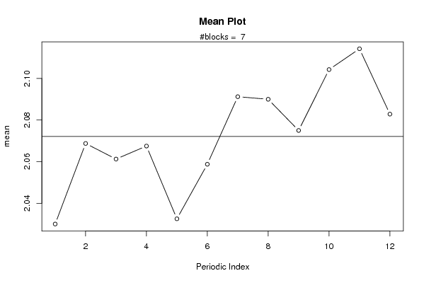
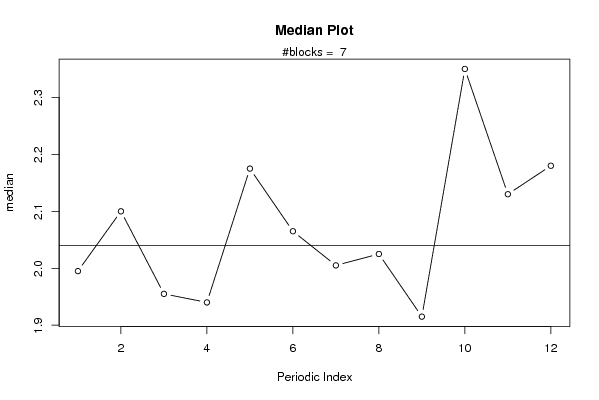
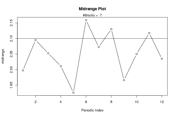
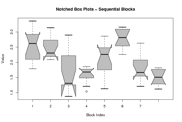
| R Software Module | rwasp_meanplot.wasp | ||||||||||||||||||||
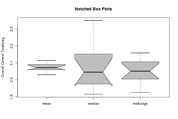
| Title produced by software | Mean Plot | ||||||||||||||||||||
| Date of computation | Fri, 26 Oct 2007 05:26:07 -0700 | ||||||||||||||||||||
| Cite this page as follows | Statistical Computations at FreeStatistics.org, Office for Research Development and Education, URL https://freestatistics.org/blog/index.php?v=date/2007/Oct/26/o8vu0wr2g9v38bh1193401198.htm/, Retrieved Mon, 29 Apr 2024 05:12:39 +0000 | ||||||||||||||||||||
| Statistical Computations at FreeStatistics.org, Office for Research Development and Education, URL https://freestatistics.org/blog/index.php?pk=1884, Retrieved Mon, 29 Apr 2024 05:12:39 +0000 | |||||||||||||||||||||
| QR Codes: | |||||||||||||||||||||
|
| |||||||||||||||||||||
| Original text written by user: | |||||||||||||||||||||
| IsPrivate? | No (this computation is public) | ||||||||||||||||||||
| User-defined keywords | opdr 3 part 1 q5 mean plot, cons prijzen | ||||||||||||||||||||
| Estimated Impact | 158 | ||||||||||||||||||||
Tree of Dependent Computations | |||||||||||||||||||||
| Family? (F = Feedback message, R = changed R code, M = changed R Module, P = changed Parameters, D = changed Data) | |||||||||||||||||||||
| - [Mean Plot] [opdr 3 part 1 q5] [2007-10-26 12:26:07] [0c12eff582f43eaf43ae2f09e879befe] [Current] | |||||||||||||||||||||
| Feedback Forum | |||||||||||||||||||||
Post a new message | |||||||||||||||||||||
Dataset | |||||||||||||||||||||
| Dataseries X: | |||||||||||||||||||||
1,79 1,95 2,26 2,04 2,16 2,75 2,79 2,88 3,36 2,97 3,1 2,49 2,2 2,25 2,09 2,79 3,14 2,93 2,65 2,67 2,26 2,35 2,13 2,18 2,9 2,63 2,67 1,81 1,33 0,88 1,28 1,26 1,26 1,29 1,1 1,37 1,21 1,74 1,76 1,48 1,04 1,62 1,49 1,79 1,8 1,58 1,86 1,74 1,59 1,26 1,13 1,92 2,61 2,26 2,41 2,26 2,03 2,86 2,55 2,27 2,26 2,57 3,07 2,76 2,51 2,87 3,14 3,11 3,16 2,47 2,57 2,89 2,63 2,38 1,69 1,96 2,19 1,87 1,6 1,63 1,22 1,21 1,49 1,64 1,66 1,77 1,82 1,78 1,28 1,29 1,37 1,12 1,51 | |||||||||||||||||||||
Tables (Output of Computation) | |||||||||||||||||||||
| |||||||||||||||||||||
Figures (Output of Computation) | |||||||||||||||||||||
Input Parameters & R Code | |||||||||||||||||||||
| Parameters (Session): | |||||||||||||||||||||
| Parameters (R input): | |||||||||||||||||||||
| par1 = 12 ; | |||||||||||||||||||||
| R code (references can be found in the software module): | |||||||||||||||||||||
par1 <- as.numeric(par1) | |||||||||||||||||||||