Free Statistics
of Irreproducible Research!
Description of Statistical Computation | |||||||||||||||||||||
|---|---|---|---|---|---|---|---|---|---|---|---|---|---|---|---|---|---|---|---|---|---|
| Author's title | |||||||||||||||||||||
| Author | *Unverified author* | ||||||||||||||||||||
| R Software Module | rwasp_backtobackhist.wasp | ||||||||||||||||||||
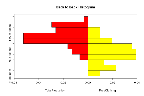
| Title produced by software | Back to Back Histogram | ||||||||||||||||||||
| Date of computation | Mon, 22 Oct 2007 01:10:57 -0700 | ||||||||||||||||||||
| Cite this page as follows | Statistical Computations at FreeStatistics.org, Office for Research Development and Education, URL https://freestatistics.org/blog/index.php?v=date/2007/Oct/22/ip6oqhcd2ea0b2v1193041528.htm/, Retrieved Mon, 06 May 2024 09:23:34 +0000 | ||||||||||||||||||||
| Statistical Computations at FreeStatistics.org, Office for Research Development and Education, URL https://freestatistics.org/blog/index.php?pk=1494, Retrieved Mon, 06 May 2024 09:23:34 +0000 | |||||||||||||||||||||
| QR Codes: | |||||||||||||||||||||
|
| |||||||||||||||||||||
| Original text written by user: | We zien in het Back-to-Back Histogram dat de Totale Productie en de Productie van Kledij verdeeld is in verschillende klassen. We merken op dat de Productie van Kledij gecentreerd is in de lager liggende klassen terwijl de Totale Productie hoofdzakelijk terug te vinden is in de hogere klassen. Dit lijkt ons vrij logisch, aangezien kledij-productie slechts een onderdeel vormt van de totale productie. | ||||||||||||||||||||
| IsPrivate? | No (this computation is public) | ||||||||||||||||||||
| User-defined keywords | Taak2.2G19 | ||||||||||||||||||||
| Estimated Impact | 197 | ||||||||||||||||||||
Tree of Dependent Computations | |||||||||||||||||||||
| Family? (F = Feedback message, R = changed R code, M = changed R Module, P = changed Parameters, D = changed Data) | |||||||||||||||||||||
| - [Back to Back Histogram] [Distributions sim...] [2007-10-22 08:10:57] [6b5c00822e2ce0f7cf73539c28d95782] [Current] | |||||||||||||||||||||
| Feedback Forum | |||||||||||||||||||||
Post a new message | |||||||||||||||||||||
Dataset | |||||||||||||||||||||
| Dataseries X: | |||||||||||||||||||||
110,40 96,40 101,90 106,20 81,00 94,70 101,00 109,40 102,30 90,70 96,20 96,10 106,00 103,10 102,00 104,70 86,00 92,10 106,90 112,60 101,70 92,00 97,40 97,00 105,40 102,70 98,10 104,50 87,40 89,90 109,80 111,70 98,60 96,90 95,10 97,00 112,70 102,90 97,40 111,40 87,40 96,80 114,10 110,30 103,90 101,60 94,60 95,90 104,70 102,80 98,10 113,90 80,90 95,70 113,20 105,90 108,80 102,30 99,00 100,70 115,50 | |||||||||||||||||||||
| Dataseries Y: | |||||||||||||||||||||
109,20 88,60 94,30 98,30 86,40 80,60 104,10 108,20 93,40 71,90 94,10 94,90 96,40 91,10 84,40 86,40 88,00 75,10 109,70 103,00 82,10 68,00 96,40 94,30 90,00 88,00 76,10 82,50 81,40 66,50 97,20 94,10 80,70 70,50 87,80 89,50 99,60 84,20 75,10 92,00 80,80 73,10 99,80 90,00 83,10 72,40 78,80 87,30 91,00 80,10 73,60 86,40 74,50 71,20 92,40 81,50 85,30 69,90 84,20 90,70 100,30 | |||||||||||||||||||||
Tables (Output of Computation) | |||||||||||||||||||||
| |||||||||||||||||||||
Figures (Output of Computation) | |||||||||||||||||||||
Input Parameters & R Code | |||||||||||||||||||||
| Parameters (Session): | |||||||||||||||||||||
| par1 = red ; par2 = yellow ; par3 = TRUE ; par4 = TotalProduction ; par5 = ProdClothing ; | |||||||||||||||||||||
| Parameters (R input): | |||||||||||||||||||||
| par1 = red ; par2 = yellow ; par3 = TRUE ; par4 = TotalProduction ; par5 = ProdClothing ; | |||||||||||||||||||||
| R code (references can be found in the software module): | |||||||||||||||||||||
if (par3 == 'TRUE') par3 <- TRUE | |||||||||||||||||||||