Free Statistics
of Irreproducible Research!
Description of Statistical Computation | |||||||||||||||||||||||||||||||||||||||||||||||||||||||||||||||||||||||||||||||||||||||||||||||||||
|---|---|---|---|---|---|---|---|---|---|---|---|---|---|---|---|---|---|---|---|---|---|---|---|---|---|---|---|---|---|---|---|---|---|---|---|---|---|---|---|---|---|---|---|---|---|---|---|---|---|---|---|---|---|---|---|---|---|---|---|---|---|---|---|---|---|---|---|---|---|---|---|---|---|---|---|---|---|---|---|---|---|---|---|---|---|---|---|---|---|---|---|---|---|---|---|---|---|---|---|
| Author's title | |||||||||||||||||||||||||||||||||||||||||||||||||||||||||||||||||||||||||||||||||||||||||||||||||||
| Author | *Unverified author* | ||||||||||||||||||||||||||||||||||||||||||||||||||||||||||||||||||||||||||||||||||||||||||||||||||
| R Software Module | rwasp_correlation.wasp | ||||||||||||||||||||||||||||||||||||||||||||||||||||||||||||||||||||||||||||||||||||||||||||||||||
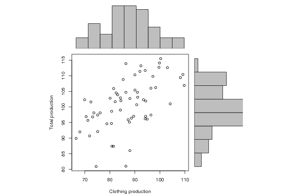
| Title produced by software | Pearson Correlation | ||||||||||||||||||||||||||||||||||||||||||||||||||||||||||||||||||||||||||||||||||||||||||||||||||
| Date of computation | Sat, 20 Oct 2007 07:22:11 -0700 | ||||||||||||||||||||||||||||||||||||||||||||||||||||||||||||||||||||||||||||||||||||||||||||||||||
| Cite this page as follows | Statistical Computations at FreeStatistics.org, Office for Research Development and Education, URL https://freestatistics.org/blog/index.php?v=date/2007/Oct/20/30u76j2iqumdtuj1192890044.htm/, Retrieved Thu, 02 May 2024 17:22:40 +0000 | ||||||||||||||||||||||||||||||||||||||||||||||||||||||||||||||||||||||||||||||||||||||||||||||||||
| Statistical Computations at FreeStatistics.org, Office for Research Development and Education, URL https://freestatistics.org/blog/index.php?pk=1094, Retrieved Thu, 02 May 2024 17:22:40 +0000 | |||||||||||||||||||||||||||||||||||||||||||||||||||||||||||||||||||||||||||||||||||||||||||||||||||
| QR Codes: | |||||||||||||||||||||||||||||||||||||||||||||||||||||||||||||||||||||||||||||||||||||||||||||||||||
|
| |||||||||||||||||||||||||||||||||||||||||||||||||||||||||||||||||||||||||||||||||||||||||||||||||||
| Original text written by user: | |||||||||||||||||||||||||||||||||||||||||||||||||||||||||||||||||||||||||||||||||||||||||||||||||||
| IsPrivate? | No (this computation is public) | ||||||||||||||||||||||||||||||||||||||||||||||||||||||||||||||||||||||||||||||||||||||||||||||||||
| User-defined keywords | Q3 juist | ||||||||||||||||||||||||||||||||||||||||||||||||||||||||||||||||||||||||||||||||||||||||||||||||||
| Estimated Impact | 488 | ||||||||||||||||||||||||||||||||||||||||||||||||||||||||||||||||||||||||||||||||||||||||||||||||||
Tree of Dependent Computations | |||||||||||||||||||||||||||||||||||||||||||||||||||||||||||||||||||||||||||||||||||||||||||||||||||
| Family? (F = Feedback message, R = changed R code, M = changed R Module, P = changed Parameters, D = changed Data) | |||||||||||||||||||||||||||||||||||||||||||||||||||||||||||||||||||||||||||||||||||||||||||||||||||
| F [Pearson Correlation] [Q3 Clothing produ...] [2007-10-20 14:22:11] [1a83104d28786df2e24859e2e02dc234] [Current] F D [Pearson Correlation] [Q3 - Clothing pro...] [2008-10-15 17:45:30] [a57f5cc542637534b8bb5bcb4d37eab1] F D [Pearson Correlation] [Correlatie kledij...] [2008-10-15 18:29:08] [8f802de8cb3f2f7005fd796d72a00b6d] - R D [Pearson Correlation] [clothing prod ass...] [2008-10-17 11:56:13] [3d2d096cc21c6f80db3dd7b8e12effce] - R D [Pearson Correlation] [Tot prod associat...] [2008-10-17 12:04:32] [3d2d096cc21c6f80db3dd7b8e12effce] - R D [Pearson Correlation] [clothing and inve...] [2008-10-17 12:07:40] [3d2d096cc21c6f80db3dd7b8e12effce] - D [Pearson Correlation] [Q3: Is Clothing P...] [2008-10-17 12:22:55] [1e1d8320a8a1170c475bf6e4ce119de6] - D [Pearson Correlation] [Pearson Correlation] [2008-10-17 13:16:06] [252acdb58d8522ab27f61fa1e87b5efe] F D [Pearson Correlation] [Verband tussen pr...] [2008-10-20 13:40:55] [1376d48f59a7212e8dd85a587491a69b] F D [Pearson Correlation] [Overeenkomst tota...] [2008-10-17 14:47:32] [cf45c678b7899ee33d7b061948f80651] - D [Pearson Correlation] [Relatie aantal ge...] [2008-10-17 17:40:27] [c45c87b96bbf32ffc2144fc37d767b2e] - D [Pearson Correlation] [relatie aantal ge...] [2008-10-17 17:44:05] [c45c87b96bbf32ffc2144fc37d767b2e] - D [Pearson Correlation] [relatie aantal ge...] [2008-10-17 17:46:26] [c45c87b96bbf32ffc2144fc37d767b2e] - D [Pearson Correlation] [investigating ass...] [2008-10-17 18:17:39] [ec1c727838a7caf353f22e99d242fe74] F RM D [Kendall tau Rank Correlation] [investigating ass...] [2008-10-17 19:07:36] [cbd3d88cd5aad6543e769146e7e26b0c] F D [Pearson Correlation] [investigating ass...] [2008-10-17 19:17:41] [cbd3d88cd5aad6543e769146e7e26b0c] F RM [Kendall tau Rank Correlation] [investigating ass...] [2008-10-17 19:35:42] [cbd3d88cd5aad6543e769146e7e26b0c] F D [Pearson Correlation] [Correlatie] [2008-10-17 21:12:26] [8b0d202c3a0c4ea223fd8b8e731dacd8] - R D [Pearson Correlation] [Q3] [2008-10-18 11:21:34] [529a65e524c481ca1098665a9566b89f] - R D [Pearson Correlation] [Q4] [2008-10-18 11:25:59] [529a65e524c481ca1098665a9566b89f] F R D [Pearson Correlation] [Q5] [2008-10-18 11:29:27] [529a65e524c481ca1098665a9566b89f] - RM D [Percentiles] [Q6] [2008-10-18 11:33:35] [529a65e524c481ca1098665a9566b89f] - RMPD [Harrell-Davis Quantiles] [Q7] [2008-10-18 11:43:23] [529a65e524c481ca1098665a9566b89f] - D [Pearson Correlation] [Correlatie kledin...] [2008-10-18 13:48:33] [d32f94eec6fe2d8c421bd223368a5ced] - D [Pearson Correlation] [Pearson correlati...] [2008-10-18 16:08:45] [b943bd7078334192ff8343563ee31113] F D [Pearson Correlation] [Correlation] [2008-10-19 08:41:50] [4396f984ebeab43316cd6baa88a4fd40] F D [Pearson Correlation] [Investigating Ass...] [2008-10-19 09:13:09] [6743688719638b0cb1c0a6e0bf433315] F D [Pearson Correlation] [Task 1 - Q3 - Clo...] [2008-10-19 10:54:35] [33f4701c7363e8b81858dafbf0350eed] - RM D [Kendall tau Rank Correlation] [Q3 association] [2008-10-19 12:01:15] [e5d91604aae608e98a8ea24759233f66] - RM D [Spearman Rank Correlation] [Q3: Spearman] [2008-10-19 12:23:25] [e5d91604aae608e98a8ea24759233f66] F D [Pearson Correlation] [Reproduction Q2] [2008-10-19 13:09:35] [86761fc994bdf34e4f4ab5b8e1d9e1c3] - D [Pearson Correlation] [Controle: Associa...] [2008-10-19 15:53:38] [5e74953d94072114d25d7276793b561e] F D [Pearson Correlation] [Pearson] [2008-10-19 16:47:00] [8d78428855b119373cac369316c08983] - RM D [Kendall tau Rank Correlation] [Kendall Tau Rank] [2008-10-19 16:51:45] [8d78428855b119373cac369316c08983] F D [Pearson Correlation] [Q3 Correlatie Tot...] [2008-10-19 17:07:54] [cf9c64468d04c2c4dd548cc66b4e3677] - D [Pearson Correlation] [Clothing Producti...] [2008-10-19 19:22:05] [988ab43f527fc78aae41c84649095267] - D [Pearson Correlation] [Is Clothing Produ...] [2008-10-19 19:51:15] [988ab43f527fc78aae41c84649095267] F D [Pearson Correlation] [Is there a relati...] [2008-10-19 19:53:05] [988ab43f527fc78aae41c84649095267] - RM D [Percentiles] [: Compute a and b...] [2008-10-19 19:55:16] [988ab43f527fc78aae41c84649095267] - RMPD [Harrell-Davis Quantiles] [Compute the 95% C...] [2008-10-19 19:58:52] [988ab43f527fc78aae41c84649095267] - PD [Harrell-Davis Quantiles] [Compute the 95% C...] [2008-10-20 15:16:26] [988ab43f527fc78aae41c84649095267] - RMPD [Univariate Data Series] [actual values of ...] [2008-10-20 15:34:58] [988ab43f527fc78aae41c84649095267] - PD [Harrell-Davis Quantiles] [New 95%] [2008-10-20 15:40:05] [988ab43f527fc78aae41c84649095267] - RMPD [Central Tendency] [Frankrijk/Uitvoer ] [2008-10-20 15:56:26] [988ab43f527fc78aae41c84649095267] - RMPD [Central Tendency] [Luxemburg/Uitvoer] [2008-10-20 15:59:18] [988ab43f527fc78aae41c84649095267] - RMPD [Central Tendency] [Nederland.Uitvoer] [2008-10-20 16:01:01] [988ab43f527fc78aae41c84649095267] - RMPD [Central Tendency] [Duitsland.Uitvoer] [2008-10-20 16:03:46] [988ab43f527fc78aae41c84649095267] F D [Pearson Correlation] [Q3 Pearson Correl...] [2008-10-20 09:12:24] [38f43994ada0e6172896e12525dcc585] F D [Pearson Correlation] [Q3 correlation] [2008-10-20 11:58:00] [dd679c9a7f849ed0333823e9c020c5a6] [Truncated] | |||||||||||||||||||||||||||||||||||||||||||||||||||||||||||||||||||||||||||||||||||||||||||||||||||
| Feedback Forum | |||||||||||||||||||||||||||||||||||||||||||||||||||||||||||||||||||||||||||||||||||||||||||||||||||
Post a new message | |||||||||||||||||||||||||||||||||||||||||||||||||||||||||||||||||||||||||||||||||||||||||||||||||||
Dataset | |||||||||||||||||||||||||||||||||||||||||||||||||||||||||||||||||||||||||||||||||||||||||||||||||||
| Dataseries X: | |||||||||||||||||||||||||||||||||||||||||||||||||||||||||||||||||||||||||||||||||||||||||||||||||||
109,20 88,60 94,30 98,30 86,40 80,60 104,10 108,20 93,40 71,90 94,10 94,90 96,40 91,10 84,40 86,40 88,00 75,10 109,70 103,00 82,10 68,00 96,40 94,30 90,00 88,00 76,10 82,50 81,40 66,50 97,20 94,10 80,70 70,50 87,80 89,50 99,60 84,20 75,10 92,00 80,80 73,10 99,80 90,00 83,10 72,40 78,80 87,30 91,00 80,10 73,60 86,40 74,50 71,20 92,40 81,50 85,30 69,90 84,20 90,70 100,30 | |||||||||||||||||||||||||||||||||||||||||||||||||||||||||||||||||||||||||||||||||||||||||||||||||||
| Dataseries Y: | |||||||||||||||||||||||||||||||||||||||||||||||||||||||||||||||||||||||||||||||||||||||||||||||||||
110,40 96,40 101,90 106,20 81,00 94,70 101,00 109,40 102,30 90,70 96,20 96,10 106,00 103,10 102,00 104,70 86,00 92,10 106,90 112,60 101,70 92,00 97,40 97,00 105,40 102,70 98,10 104,50 87,40 89,90 109,80 111,70 98,60 96,90 95,10 97,00 112,70 102,90 97,40 111,40 87,40 96,80 114,10 110,30 103,90 101,60 94,60 95,90 104,70 102,80 98,10 113,90 80,90 95,70 113,20 105,90 108,80 102,30 99,00 100,70 115,50 | |||||||||||||||||||||||||||||||||||||||||||||||||||||||||||||||||||||||||||||||||||||||||||||||||||
Tables (Output of Computation) | |||||||||||||||||||||||||||||||||||||||||||||||||||||||||||||||||||||||||||||||||||||||||||||||||||
| |||||||||||||||||||||||||||||||||||||||||||||||||||||||||||||||||||||||||||||||||||||||||||||||||||
Figures (Output of Computation) | |||||||||||||||||||||||||||||||||||||||||||||||||||||||||||||||||||||||||||||||||||||||||||||||||||
Input Parameters & R Code | |||||||||||||||||||||||||||||||||||||||||||||||||||||||||||||||||||||||||||||||||||||||||||||||||||
| Parameters (Session): | |||||||||||||||||||||||||||||||||||||||||||||||||||||||||||||||||||||||||||||||||||||||||||||||||||
| Parameters (R input): | |||||||||||||||||||||||||||||||||||||||||||||||||||||||||||||||||||||||||||||||||||||||||||||||||||
| R code (references can be found in the software module): | |||||||||||||||||||||||||||||||||||||||||||||||||||||||||||||||||||||||||||||||||||||||||||||||||||
bitmap(file='test1.png') | |||||||||||||||||||||||||||||||||||||||||||||||||||||||||||||||||||||||||||||||||||||||||||||||||||