Repository of Reproducible Computations

Free Statistics

of Irreproducible Research!

Author's title

Author

*Unverified author*

R Software Module

rwasp_autocorrelation.wasp

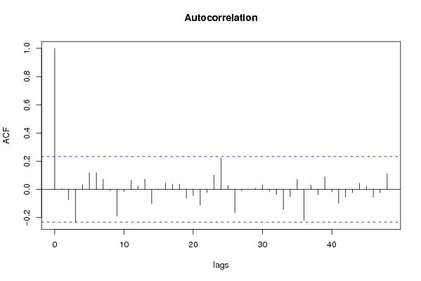
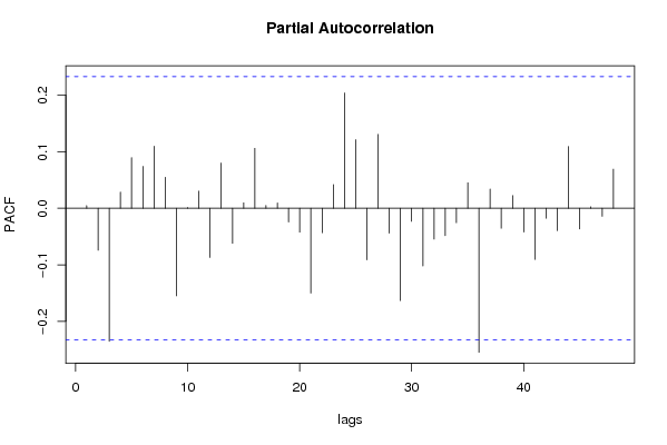
Title produced by software

(Partial) Autocorrelation Function

Date of computation

Fri, 30 Nov 2007 07:06:24 -0700

Cite this page as follows

Statistical Computations at FreeStatistics.org, Office for Research Development and Education, URL https://freestatistics.org/blog/index.php?v=date/2007/Nov/30/t1196430967xbqtgmnb8onxv6x.htm/, Retrieved Sat, 27 Apr 2024 22:42:42 +0000

Statistical Computations at FreeStatistics.org, Office for Research Development and Education, URL https://freestatistics.org/blog/index.php?pk=7690, Retrieved Sat, 27 Apr 2024 22:42:42 +0000

QR Codes:

Paste this QR Code to cite your computation.

Original text written by user:

IsPrivate?

No (this computation is public)

User-defined keywords

Estimated Impact

201

Family? (F = Feedback message, R = changed R code, M = changed R Module, P = changed Parameters, D = changed Data)

-       [(Partial) Autocorrelation Function] [] [2007-11-30 14:06:24] [a1fadf46580e43815db2830b4560d35f] [Current]

Feedback Forum

Post a new message

Dataseries X:

Download CSV

Histogram

Boxplots

Summary of compuational transaction
Raw Input	view raw input (R code)
Raw Output	view raw output of R engine
Computing time	1 seconds
R Server	'Gwilym Jenkins' @ 72.249.127.135

\begin{tabular}{lllllllll}
\hline
Summary of compuational transaction \tabularnewline
Raw Input & view raw input (R code)  \tabularnewline
Raw Output & view raw output of R engine  \tabularnewline
Computing time & 1 seconds \tabularnewline
R Server & 'Gwilym Jenkins' @ 72.249.127.135 \tabularnewline
\hline
\end{tabular}
%Source: https://freestatistics.org/blog/index.php?pk=7690&T=0

[TABLE]
[ROW][C]Summary of compuational transaction[/C][/ROW]
[ROW][C]Raw Input[/C][C]view raw input (R code) [/C][/ROW]
[ROW][C]Raw Output[/C][C]view raw output of R engine [/C][/ROW]
[ROW][C]Computing time[/C][C]1 seconds[/C][/ROW]
[ROW][C]R Server[/C][C]'Gwilym Jenkins' @ 72.249.127.135[/C][/ROW]
[/TABLE]
Source: https://freestatistics.org/blog/index.php?pk=7690&T=0

Globally Unique Identifier (entire table): ba.freestatistics.org/blog/index.php?pk=7690&T=0

As an alternative you can also use a QR Code:

The GUIDs for individual cells are displayed in the table below:

Summary of compuational transaction
Raw Input	view raw input (R code)
Raw Output	view raw output of R engine
Computing time	1 seconds
R Server	'Gwilym Jenkins' @ 72.249.127.135

Autocorrelation Function
Time lag k	ACF(k)	T-STAT	P-value
0	1	8.4261	0
1	0.004584	0.0386	0.484649
2	-0.07428	-0.6259	0.733305
3	-0.234657	-1.9773	0.974052
4	0.034098	0.2873	0.387354
5	0.11801	0.9944	0.16171
6	0.118232	0.9962	0.161258
7	0.072288	0.6091	0.272197
8	-0.01003	-0.0845	0.533556
9	-0.188507	-1.5884	0.941679
10	-0.014245	-0.12	0.547602
11	0.065735	0.5539	0.290697
12	0.02358	0.1987	0.421537
13	0.07138	0.6015	0.274724
14	-0.101961	-0.8591	0.803422
15	-0.002801	-0.0236	0.509381
16	0.044284	0.3731	0.355076
17	0.037211	0.3135	0.377391
18	0.036247	0.3054	0.380469
19	-0.061564	-0.5187	0.697224
20	-0.043958	-0.3704	0.643904
21	-0.112908	-0.9514	0.82768
22	-0.022542	-0.1899	0.57505
23	0.100741	0.8489	0.199406
24	0.22049	1.8579	0.033666
25	0.027573	0.2323	0.408475
26	-0.166996	-1.4071	0.918124
27	-0.010716	-0.0903	0.535845
28	-0.001696	-0.0143	0.50568
29	0.008814	0.0743	0.470502
30	0.032351	0.2726	0.392978
31	-0.014222	-0.1198	0.547525
32	-0.035491	-0.2991	0.617113
33	-0.141679	-1.1938	0.881737
34	-0.051786	-0.4364	0.668049
35	0.071218	0.6001	0.275176
36	-0.219669	-1.851	0.965833
37	0.031235	0.2632	0.396583
38	-0.039529	-0.3331	0.62997
39	0.090109	0.7593	0.225102
40	-0.016202	-0.1365	0.554102
41	-0.099154	-0.8355	0.796877
42	-0.055897	-0.471	0.680456
43	-0.022637	-0.1907	0.575363
44	0.043708	0.3683	0.356877
45	0.022886	0.1928	0.423817
46	-0.056404	-0.4753	0.681971
47	-0.024725	-0.2083	0.58222

\begin{tabular}{lllllllll}
\hline
Autocorrelation Function \tabularnewline
Time lag k & ACF(k) & T-STAT & P-value \tabularnewline
0 & 1 & 8.4261 & 0 \tabularnewline
1 & 0.004584 & 0.0386 & 0.484649 \tabularnewline
2 & -0.07428 & -0.6259 & 0.733305 \tabularnewline
3 & -0.234657 & -1.9773 & 0.974052 \tabularnewline
4 & 0.034098 & 0.2873 & 0.387354 \tabularnewline
5 & 0.11801 & 0.9944 & 0.16171 \tabularnewline
6 & 0.118232 & 0.9962 & 0.161258 \tabularnewline
7 & 0.072288 & 0.6091 & 0.272197 \tabularnewline
8 & -0.01003 & -0.0845 & 0.533556 \tabularnewline
9 & -0.188507 & -1.5884 & 0.941679 \tabularnewline
10 & -0.014245 & -0.12 & 0.547602 \tabularnewline
11 & 0.065735 & 0.5539 & 0.290697 \tabularnewline
12 & 0.02358 & 0.1987 & 0.421537 \tabularnewline
13 & 0.07138 & 0.6015 & 0.274724 \tabularnewline
14 & -0.101961 & -0.8591 & 0.803422 \tabularnewline
15 & -0.002801 & -0.0236 & 0.509381 \tabularnewline
16 & 0.044284 & 0.3731 & 0.355076 \tabularnewline
17 & 0.037211 & 0.3135 & 0.377391 \tabularnewline
18 & 0.036247 & 0.3054 & 0.380469 \tabularnewline
19 & -0.061564 & -0.5187 & 0.697224 \tabularnewline
20 & -0.043958 & -0.3704 & 0.643904 \tabularnewline
21 & -0.112908 & -0.9514 & 0.82768 \tabularnewline
22 & -0.022542 & -0.1899 & 0.57505 \tabularnewline
23 & 0.100741 & 0.8489 & 0.199406 \tabularnewline
24 & 0.22049 & 1.8579 & 0.033666 \tabularnewline
25 & 0.027573 & 0.2323 & 0.408475 \tabularnewline
26 & -0.166996 & -1.4071 & 0.918124 \tabularnewline
27 & -0.010716 & -0.0903 & 0.535845 \tabularnewline
28 & -0.001696 & -0.0143 & 0.50568 \tabularnewline
29 & 0.008814 & 0.0743 & 0.470502 \tabularnewline
30 & 0.032351 & 0.2726 & 0.392978 \tabularnewline
31 & -0.014222 & -0.1198 & 0.547525 \tabularnewline
32 & -0.035491 & -0.2991 & 0.617113 \tabularnewline
33 & -0.141679 & -1.1938 & 0.881737 \tabularnewline
34 & -0.051786 & -0.4364 & 0.668049 \tabularnewline
35 & 0.071218 & 0.6001 & 0.275176 \tabularnewline
36 & -0.219669 & -1.851 & 0.965833 \tabularnewline
37 & 0.031235 & 0.2632 & 0.396583 \tabularnewline
38 & -0.039529 & -0.3331 & 0.62997 \tabularnewline
39 & 0.090109 & 0.7593 & 0.225102 \tabularnewline
40 & -0.016202 & -0.1365 & 0.554102 \tabularnewline
41 & -0.099154 & -0.8355 & 0.796877 \tabularnewline
42 & -0.055897 & -0.471 & 0.680456 \tabularnewline
43 & -0.022637 & -0.1907 & 0.575363 \tabularnewline
44 & 0.043708 & 0.3683 & 0.356877 \tabularnewline
45 & 0.022886 & 0.1928 & 0.423817 \tabularnewline
46 & -0.056404 & -0.4753 & 0.681971 \tabularnewline
47 & -0.024725 & -0.2083 & 0.58222 \tabularnewline
\hline
\end{tabular}
%Source: https://freestatistics.org/blog/index.php?pk=7690&T=1

[TABLE]
[ROW][C]Autocorrelation Function[/C][/ROW]
[ROW][C]Time lag k[/C][C]ACF(k)[/C][C]T-STAT[/C][C]P-value[/C][/ROW]
[ROW][C]0[/C][C]1[/C][C]8.4261[/C][C]0[/C][/ROW]
[ROW][C]1[/C][C]0.004584[/C][C]0.0386[/C][C]0.484649[/C][/ROW]
[ROW][C]2[/C][C]-0.07428[/C][C]-0.6259[/C][C]0.733305[/C][/ROW]
[ROW][C]3[/C][C]-0.234657[/C][C]-1.9773[/C][C]0.974052[/C][/ROW]
[ROW][C]4[/C][C]0.034098[/C][C]0.2873[/C][C]0.387354[/C][/ROW]
[ROW][C]5[/C][C]0.11801[/C][C]0.9944[/C][C]0.16171[/C][/ROW]
[ROW][C]6[/C][C]0.118232[/C][C]0.9962[/C][C]0.161258[/C][/ROW]
[ROW][C]7[/C][C]0.072288[/C][C]0.6091[/C][C]0.272197[/C][/ROW]
[ROW][C]8[/C][C]-0.01003[/C][C]-0.0845[/C][C]0.533556[/C][/ROW]
[ROW][C]9[/C][C]-0.188507[/C][C]-1.5884[/C][C]0.941679[/C][/ROW]
[ROW][C]10[/C][C]-0.014245[/C][C]-0.12[/C][C]0.547602[/C][/ROW]
[ROW][C]11[/C][C]0.065735[/C][C]0.5539[/C][C]0.290697[/C][/ROW]
[ROW][C]12[/C][C]0.02358[/C][C]0.1987[/C][C]0.421537[/C][/ROW]
[ROW][C]13[/C][C]0.07138[/C][C]0.6015[/C][C]0.274724[/C][/ROW]
[ROW][C]14[/C][C]-0.101961[/C][C]-0.8591[/C][C]0.803422[/C][/ROW]
[ROW][C]15[/C][C]-0.002801[/C][C]-0.0236[/C][C]0.509381[/C][/ROW]
[ROW][C]16[/C][C]0.044284[/C][C]0.3731[/C][C]0.355076[/C][/ROW]
[ROW][C]17[/C][C]0.037211[/C][C]0.3135[/C][C]0.377391[/C][/ROW]
[ROW][C]18[/C][C]0.036247[/C][C]0.3054[/C][C]0.380469[/C][/ROW]
[ROW][C]19[/C][C]-0.061564[/C][C]-0.5187[/C][C]0.697224[/C][/ROW]
[ROW][C]20[/C][C]-0.043958[/C][C]-0.3704[/C][C]0.643904[/C][/ROW]
[ROW][C]21[/C][C]-0.112908[/C][C]-0.9514[/C][C]0.82768[/C][/ROW]
[ROW][C]22[/C][C]-0.022542[/C][C]-0.1899[/C][C]0.57505[/C][/ROW]
[ROW][C]23[/C][C]0.100741[/C][C]0.8489[/C][C]0.199406[/C][/ROW]
[ROW][C]24[/C][C]0.22049[/C][C]1.8579[/C][C]0.033666[/C][/ROW]
[ROW][C]25[/C][C]0.027573[/C][C]0.2323[/C][C]0.408475[/C][/ROW]
[ROW][C]26[/C][C]-0.166996[/C][C]-1.4071[/C][C]0.918124[/C][/ROW]
[ROW][C]27[/C][C]-0.010716[/C][C]-0.0903[/C][C]0.535845[/C][/ROW]
[ROW][C]28[/C][C]-0.001696[/C][C]-0.0143[/C][C]0.50568[/C][/ROW]
[ROW][C]29[/C][C]0.008814[/C][C]0.0743[/C][C]0.470502[/C][/ROW]
[ROW][C]30[/C][C]0.032351[/C][C]0.2726[/C][C]0.392978[/C][/ROW]
[ROW][C]31[/C][C]-0.014222[/C][C]-0.1198[/C][C]0.547525[/C][/ROW]
[ROW][C]32[/C][C]-0.035491[/C][C]-0.2991[/C][C]0.617113[/C][/ROW]
[ROW][C]33[/C][C]-0.141679[/C][C]-1.1938[/C][C]0.881737[/C][/ROW]
[ROW][C]34[/C][C]-0.051786[/C][C]-0.4364[/C][C]0.668049[/C][/ROW]
[ROW][C]35[/C][C]0.071218[/C][C]0.6001[/C][C]0.275176[/C][/ROW]
[ROW][C]36[/C][C]-0.219669[/C][C]-1.851[/C][C]0.965833[/C][/ROW]
[ROW][C]37[/C][C]0.031235[/C][C]0.2632[/C][C]0.396583[/C][/ROW]
[ROW][C]38[/C][C]-0.039529[/C][C]-0.3331[/C][C]0.62997[/C][/ROW]
[ROW][C]39[/C][C]0.090109[/C][C]0.7593[/C][C]0.225102[/C][/ROW]
[ROW][C]40[/C][C]-0.016202[/C][C]-0.1365[/C][C]0.554102[/C][/ROW]
[ROW][C]41[/C][C]-0.099154[/C][C]-0.8355[/C][C]0.796877[/C][/ROW]
[ROW][C]42[/C][C]-0.055897[/C][C]-0.471[/C][C]0.680456[/C][/ROW]
[ROW][C]43[/C][C]-0.022637[/C][C]-0.1907[/C][C]0.575363[/C][/ROW]
[ROW][C]44[/C][C]0.043708[/C][C]0.3683[/C][C]0.356877[/C][/ROW]
[ROW][C]45[/C][C]0.022886[/C][C]0.1928[/C][C]0.423817[/C][/ROW]
[ROW][C]46[/C][C]-0.056404[/C][C]-0.4753[/C][C]0.681971[/C][/ROW]
[ROW][C]47[/C][C]-0.024725[/C][C]-0.2083[/C][C]0.58222[/C][/ROW]
[/TABLE]
Source: https://freestatistics.org/blog/index.php?pk=7690&T=1

Globally Unique Identifier (entire table): ba.freestatistics.org/blog/index.php?pk=7690&T=1

As an alternative you can also use a QR Code:

The GUIDs for individual cells are displayed in the table below:

Autocorrelation Function
Time lag k	ACF(k)	T-STAT	P-value
0	1	8.4261	0
1	0.004584	0.0386	0.484649
2	-0.07428	-0.6259	0.733305
3	-0.234657	-1.9773	0.974052
4	0.034098	0.2873	0.387354
5	0.11801	0.9944	0.16171
6	0.118232	0.9962	0.161258
7	0.072288	0.6091	0.272197
8	-0.01003	-0.0845	0.533556
9	-0.188507	-1.5884	0.941679
10	-0.014245	-0.12	0.547602
11	0.065735	0.5539	0.290697
12	0.02358	0.1987	0.421537
13	0.07138	0.6015	0.274724
14	-0.101961	-0.8591	0.803422
15	-0.002801	-0.0236	0.509381
16	0.044284	0.3731	0.355076
17	0.037211	0.3135	0.377391
18	0.036247	0.3054	0.380469
19	-0.061564	-0.5187	0.697224
20	-0.043958	-0.3704	0.643904
21	-0.112908	-0.9514	0.82768
22	-0.022542	-0.1899	0.57505
23	0.100741	0.8489	0.199406
24	0.22049	1.8579	0.033666
25	0.027573	0.2323	0.408475
26	-0.166996	-1.4071	0.918124
27	-0.010716	-0.0903	0.535845
28	-0.001696	-0.0143	0.50568
29	0.008814	0.0743	0.470502
30	0.032351	0.2726	0.392978
31	-0.014222	-0.1198	0.547525
32	-0.035491	-0.2991	0.617113
33	-0.141679	-1.1938	0.881737
34	-0.051786	-0.4364	0.668049
35	0.071218	0.6001	0.275176
36	-0.219669	-1.851	0.965833
37	0.031235	0.2632	0.396583
38	-0.039529	-0.3331	0.62997
39	0.090109	0.7593	0.225102
40	-0.016202	-0.1365	0.554102
41	-0.099154	-0.8355	0.796877
42	-0.055897	-0.471	0.680456
43	-0.022637	-0.1907	0.575363
44	0.043708	0.3683	0.356877
45	0.022886	0.1928	0.423817
46	-0.056404	-0.4753	0.681971
47	-0.024725	-0.2083	0.58222

Partial Autocorrelation Function
Time lag k	PACF(k)	T-STAT	P-value
0	0.004584	0.0386	0.484649
1	-0.074303	-0.6261	0.733367
2	-0.235254	-1.9823	0.974341
3	0.028525	0.2404	0.405374
4	0.089443	0.7537	0.226772
5	0.074154	0.6248	0.267041
6	0.109584	0.9234	0.17947
7	0.054732	0.4612	0.323041
8	-0.154898	-1.3052	0.901979
9	0.001167	0.0098	0.496091
10	0.030265	0.255	0.399722
11	-0.086938	-0.7326	0.766879
12	0.080014	0.6742	0.251183
13	-0.061854	-0.5212	0.698072
14	0.00965	0.0813	0.467712
15	0.105968	0.8929	0.187462
16	0.004927	0.0415	0.483502
17	0.009323	0.0786	0.468804
18	-0.024331	-0.205	0.580926
19	-0.042271	-0.3562	0.638621
20	-0.149944	-1.2635	0.89472
21	-0.043324	-0.3651	0.641922
22	0.041874	0.3528	0.362628
23	0.203802	1.7173	0.045145
24	0.12114	1.0207	0.155421
25	-0.091295	-0.7693	0.777857
26	0.130659	1.101	0.137317
27	-0.043886	-0.3698	0.643681
28	-0.163247	-1.3755	0.913356
29	-0.023133	-0.1949	0.576995
30	-0.102012	-0.8596	0.803541
31	-0.054645	-0.4604	0.676697
32	-0.048491	-0.4086	0.657966
33	-0.025463	-0.2146	0.584634
34	0.045066	0.3797	0.35264
35	-0.254639	-2.1456	0.982338
36	0.034047	0.2869	0.387517
37	-0.035297	-0.2974	0.616493
38	0.022463	0.1893	0.425209
39	-0.041928	-0.3533	0.637543
40	-0.090543	-0.7629	0.775985
41	-0.017614	-0.1484	0.558783
42	-0.039508	-0.3329	0.629904
43	0.109168	0.9199	0.180379
44	-0.036694	-0.3092	0.620958
45	0.002623	0.0221	0.491215
46	-0.014142	-0.1192	0.547258
47	0.069215	0.5832	0.280798

\begin{tabular}{lllllllll}
\hline
Partial Autocorrelation Function \tabularnewline
Time lag k & PACF(k) & T-STAT & P-value \tabularnewline
0 & 0.004584 & 0.0386 & 0.484649 \tabularnewline
1 & -0.074303 & -0.6261 & 0.733367 \tabularnewline
2 & -0.235254 & -1.9823 & 0.974341 \tabularnewline
3 & 0.028525 & 0.2404 & 0.405374 \tabularnewline
4 & 0.089443 & 0.7537 & 0.226772 \tabularnewline
5 & 0.074154 & 0.6248 & 0.267041 \tabularnewline
6 & 0.109584 & 0.9234 & 0.17947 \tabularnewline
7 & 0.054732 & 0.4612 & 0.323041 \tabularnewline
8 & -0.154898 & -1.3052 & 0.901979 \tabularnewline
9 & 0.001167 & 0.0098 & 0.496091 \tabularnewline
10 & 0.030265 & 0.255 & 0.399722 \tabularnewline
11 & -0.086938 & -0.7326 & 0.766879 \tabularnewline
12 & 0.080014 & 0.6742 & 0.251183 \tabularnewline
13 & -0.061854 & -0.5212 & 0.698072 \tabularnewline
14 & 0.00965 & 0.0813 & 0.467712 \tabularnewline
15 & 0.105968 & 0.8929 & 0.187462 \tabularnewline
16 & 0.004927 & 0.0415 & 0.483502 \tabularnewline
17 & 0.009323 & 0.0786 & 0.468804 \tabularnewline
18 & -0.024331 & -0.205 & 0.580926 \tabularnewline
19 & -0.042271 & -0.3562 & 0.638621 \tabularnewline
20 & -0.149944 & -1.2635 & 0.89472 \tabularnewline
21 & -0.043324 & -0.3651 & 0.641922 \tabularnewline
22 & 0.041874 & 0.3528 & 0.362628 \tabularnewline
23 & 0.203802 & 1.7173 & 0.045145 \tabularnewline
24 & 0.12114 & 1.0207 & 0.155421 \tabularnewline
25 & -0.091295 & -0.7693 & 0.777857 \tabularnewline
26 & 0.130659 & 1.101 & 0.137317 \tabularnewline
27 & -0.043886 & -0.3698 & 0.643681 \tabularnewline
28 & -0.163247 & -1.3755 & 0.913356 \tabularnewline
29 & -0.023133 & -0.1949 & 0.576995 \tabularnewline
30 & -0.102012 & -0.8596 & 0.803541 \tabularnewline
31 & -0.054645 & -0.4604 & 0.676697 \tabularnewline
32 & -0.048491 & -0.4086 & 0.657966 \tabularnewline
33 & -0.025463 & -0.2146 & 0.584634 \tabularnewline
34 & 0.045066 & 0.3797 & 0.35264 \tabularnewline
35 & -0.254639 & -2.1456 & 0.982338 \tabularnewline
36 & 0.034047 & 0.2869 & 0.387517 \tabularnewline
37 & -0.035297 & -0.2974 & 0.616493 \tabularnewline
38 & 0.022463 & 0.1893 & 0.425209 \tabularnewline
39 & -0.041928 & -0.3533 & 0.637543 \tabularnewline
40 & -0.090543 & -0.7629 & 0.775985 \tabularnewline
41 & -0.017614 & -0.1484 & 0.558783 \tabularnewline
42 & -0.039508 & -0.3329 & 0.629904 \tabularnewline
43 & 0.109168 & 0.9199 & 0.180379 \tabularnewline
44 & -0.036694 & -0.3092 & 0.620958 \tabularnewline
45 & 0.002623 & 0.0221 & 0.491215 \tabularnewline
46 & -0.014142 & -0.1192 & 0.547258 \tabularnewline
47 & 0.069215 & 0.5832 & 0.280798 \tabularnewline
\hline
\end{tabular}
%Source: https://freestatistics.org/blog/index.php?pk=7690&T=2

[TABLE]
[ROW][C]Partial Autocorrelation Function[/C][/ROW]
[ROW][C]Time lag k[/C][C]PACF(k)[/C][C]T-STAT[/C][C]P-value[/C][/ROW]
[ROW][C]0[/C][C]0.004584[/C][C]0.0386[/C][C]0.484649[/C][/ROW]
[ROW][C]1[/C][C]-0.074303[/C][C]-0.6261[/C][C]0.733367[/C][/ROW]
[ROW][C]2[/C][C]-0.235254[/C][C]-1.9823[/C][C]0.974341[/C][/ROW]
[ROW][C]3[/C][C]0.028525[/C][C]0.2404[/C][C]0.405374[/C][/ROW]
[ROW][C]4[/C][C]0.089443[/C][C]0.7537[/C][C]0.226772[/C][/ROW]
[ROW][C]5[/C][C]0.074154[/C][C]0.6248[/C][C]0.267041[/C][/ROW]
[ROW][C]6[/C][C]0.109584[/C][C]0.9234[/C][C]0.17947[/C][/ROW]
[ROW][C]7[/C][C]0.054732[/C][C]0.4612[/C][C]0.323041[/C][/ROW]
[ROW][C]8[/C][C]-0.154898[/C][C]-1.3052[/C][C]0.901979[/C][/ROW]
[ROW][C]9[/C][C]0.001167[/C][C]0.0098[/C][C]0.496091[/C][/ROW]
[ROW][C]10[/C][C]0.030265[/C][C]0.255[/C][C]0.399722[/C][/ROW]
[ROW][C]11[/C][C]-0.086938[/C][C]-0.7326[/C][C]0.766879[/C][/ROW]
[ROW][C]12[/C][C]0.080014[/C][C]0.6742[/C][C]0.251183[/C][/ROW]
[ROW][C]13[/C][C]-0.061854[/C][C]-0.5212[/C][C]0.698072[/C][/ROW]
[ROW][C]14[/C][C]0.00965[/C][C]0.0813[/C][C]0.467712[/C][/ROW]
[ROW][C]15[/C][C]0.105968[/C][C]0.8929[/C][C]0.187462[/C][/ROW]
[ROW][C]16[/C][C]0.004927[/C][C]0.0415[/C][C]0.483502[/C][/ROW]
[ROW][C]17[/C][C]0.009323[/C][C]0.0786[/C][C]0.468804[/C][/ROW]
[ROW][C]18[/C][C]-0.024331[/C][C]-0.205[/C][C]0.580926[/C][/ROW]
[ROW][C]19[/C][C]-0.042271[/C][C]-0.3562[/C][C]0.638621[/C][/ROW]
[ROW][C]20[/C][C]-0.149944[/C][C]-1.2635[/C][C]0.89472[/C][/ROW]
[ROW][C]21[/C][C]-0.043324[/C][C]-0.3651[/C][C]0.641922[/C][/ROW]
[ROW][C]22[/C][C]0.041874[/C][C]0.3528[/C][C]0.362628[/C][/ROW]
[ROW][C]23[/C][C]0.203802[/C][C]1.7173[/C][C]0.045145[/C][/ROW]
[ROW][C]24[/C][C]0.12114[/C][C]1.0207[/C][C]0.155421[/C][/ROW]
[ROW][C]25[/C][C]-0.091295[/C][C]-0.7693[/C][C]0.777857[/C][/ROW]
[ROW][C]26[/C][C]0.130659[/C][C]1.101[/C][C]0.137317[/C][/ROW]
[ROW][C]27[/C][C]-0.043886[/C][C]-0.3698[/C][C]0.643681[/C][/ROW]
[ROW][C]28[/C][C]-0.163247[/C][C]-1.3755[/C][C]0.913356[/C][/ROW]
[ROW][C]29[/C][C]-0.023133[/C][C]-0.1949[/C][C]0.576995[/C][/ROW]
[ROW][C]30[/C][C]-0.102012[/C][C]-0.8596[/C][C]0.803541[/C][/ROW]
[ROW][C]31[/C][C]-0.054645[/C][C]-0.4604[/C][C]0.676697[/C][/ROW]
[ROW][C]32[/C][C]-0.048491[/C][C]-0.4086[/C][C]0.657966[/C][/ROW]
[ROW][C]33[/C][C]-0.025463[/C][C]-0.2146[/C][C]0.584634[/C][/ROW]
[ROW][C]34[/C][C]0.045066[/C][C]0.3797[/C][C]0.35264[/C][/ROW]
[ROW][C]35[/C][C]-0.254639[/C][C]-2.1456[/C][C]0.982338[/C][/ROW]
[ROW][C]36[/C][C]0.034047[/C][C]0.2869[/C][C]0.387517[/C][/ROW]
[ROW][C]37[/C][C]-0.035297[/C][C]-0.2974[/C][C]0.616493[/C][/ROW]
[ROW][C]38[/C][C]0.022463[/C][C]0.1893[/C][C]0.425209[/C][/ROW]
[ROW][C]39[/C][C]-0.041928[/C][C]-0.3533[/C][C]0.637543[/C][/ROW]
[ROW][C]40[/C][C]-0.090543[/C][C]-0.7629[/C][C]0.775985[/C][/ROW]
[ROW][C]41[/C][C]-0.017614[/C][C]-0.1484[/C][C]0.558783[/C][/ROW]
[ROW][C]42[/C][C]-0.039508[/C][C]-0.3329[/C][C]0.629904[/C][/ROW]
[ROW][C]43[/C][C]0.109168[/C][C]0.9199[/C][C]0.180379[/C][/ROW]
[ROW][C]44[/C][C]-0.036694[/C][C]-0.3092[/C][C]0.620958[/C][/ROW]
[ROW][C]45[/C][C]0.002623[/C][C]0.0221[/C][C]0.491215[/C][/ROW]
[ROW][C]46[/C][C]-0.014142[/C][C]-0.1192[/C][C]0.547258[/C][/ROW]
[ROW][C]47[/C][C]0.069215[/C][C]0.5832[/C][C]0.280798[/C][/ROW]
[/TABLE]
Source: https://freestatistics.org/blog/index.php?pk=7690&T=2

Globally Unique Identifier (entire table): ba.freestatistics.org/blog/index.php?pk=7690&T=2

As an alternative you can also use a QR Code:

The GUIDs for individual cells are displayed in the table below:

Partial Autocorrelation Function
Time lag k	PACF(k)	T-STAT	P-value
0	0.004584	0.0386	0.484649
1	-0.074303	-0.6261	0.733367
2	-0.235254	-1.9823	0.974341
3	0.028525	0.2404	0.405374
4	0.089443	0.7537	0.226772
5	0.074154	0.6248	0.267041
6	0.109584	0.9234	0.17947
7	0.054732	0.4612	0.323041
8	-0.154898	-1.3052	0.901979
9	0.001167	0.0098	0.496091
10	0.030265	0.255	0.399722
11	-0.086938	-0.7326	0.766879
12	0.080014	0.6742	0.251183
13	-0.061854	-0.5212	0.698072
14	0.00965	0.0813	0.467712
15	0.105968	0.8929	0.187462
16	0.004927	0.0415	0.483502
17	0.009323	0.0786	0.468804
18	-0.024331	-0.205	0.580926
19	-0.042271	-0.3562	0.638621
20	-0.149944	-1.2635	0.89472
21	-0.043324	-0.3651	0.641922
22	0.041874	0.3528	0.362628
23	0.203802	1.7173	0.045145
24	0.12114	1.0207	0.155421
25	-0.091295	-0.7693	0.777857
26	0.130659	1.101	0.137317
27	-0.043886	-0.3698	0.643681
28	-0.163247	-1.3755	0.913356
29	-0.023133	-0.1949	0.576995
30	-0.102012	-0.8596	0.803541
31	-0.054645	-0.4604	0.676697
32	-0.048491	-0.4086	0.657966
33	-0.025463	-0.2146	0.584634
34	0.045066	0.3797	0.35264
35	-0.254639	-2.1456	0.982338
36	0.034047	0.2869	0.387517
37	-0.035297	-0.2974	0.616493
38	0.022463	0.1893	0.425209
39	-0.041928	-0.3533	0.637543
40	-0.090543	-0.7629	0.775985
41	-0.017614	-0.1484	0.558783
42	-0.039508	-0.3329	0.629904
43	0.109168	0.9199	0.180379
44	-0.036694	-0.3092	0.620958
45	0.002623	0.0221	0.491215
46	-0.014142	-0.1192	0.547258
47	0.069215	0.5832	0.280798

Figure 1

PNG link

Postscript link

PDF link

Figure 2

PNG link

Postscript link

PDF link

Parameters (Session):

par1 = 48 ; par2 = 2.0 ; par3 = 1 ; par4 = 0 ; par5 = 12 ;

Parameters (R input):

par1 = 48 ; par2 = 2.0 ; par3 = 1 ; par4 = 0 ; par5 = 12 ;

R code (references can be found in the software module):

if (par1 == 'Default') {
par1 = 10*log10(length(x))
} else {
par1 <- as.numeric(par1)
}
par2 <- as.numeric(par2)
par3 <- as.numeric(par3)
par4 <- as.numeric(par4)
par5 <- as.numeric(par5)
if (par2 == 0) {
x <- log(x)
} else {
x <- (x ^ par2 - 1) / par2
}
if (par3 > 0) x <- diff(x,lag=1,difference=par3)
if (par4 > 0) x <- diff(x,lag=par5,difference=par4)
bitmap(file='pic1.png')
racf <- acf(x,par1,main='Autocorrelation',xlab='lags',ylab='ACF')
dev.off()
bitmap(file='pic2.png')
rpacf <- pacf(x,par1,main='Partial Autocorrelation',xlab='lags',ylab='PACF')
dev.off()
(myacf <- c(racf$acf))
(mypacf <- c(rpacf$acf))
lengthx <- length(x)
sqrtn <- sqrt(lengthx)
load(file='createtable')
a<-table.start()
a<-table.row.start(a)
a<-table.element(a,'Autocorrelation Function',4,TRUE)
a<-table.row.end(a)
a<-table.row.start(a)
a<-table.element(a,'Time lag k',header=TRUE)
a<-table.element(a,hyperlink('basics.htm','ACF(k)','click here for more information about the Autocorrelation Function'),header=TRUE)
a<-table.element(a,'T-STAT',header=TRUE)
a<-table.element(a,'P-value',header=TRUE)
a<-table.row.end(a)
for (i in 1:par1) {
a<-table.row.start(a)
a<-table.element(a,i-1,header=TRUE)
a<-table.element(a,round(myacf[i],6))
mytstat <- myacf[i]*sqrtn
a<-table.element(a,round(mytstat,4))
a<-table.element(a,round(1-pt(mytstat,lengthx),6))
a<-table.row.end(a)
}
a<-table.end(a)
table.save(a,file='mytable.tab')
a<-table.start()
a<-table.row.start(a)
a<-table.element(a,'Partial Autocorrelation Function',4,TRUE)
a<-table.row.end(a)
a<-table.row.start(a)
a<-table.element(a,'Time lag k',header=TRUE)
a<-table.element(a,hyperlink('basics.htm','PACF(k)','click here for more information about the Partial Autocorrelation Function'),header=TRUE)
a<-table.element(a,'T-STAT',header=TRUE)
a<-table.element(a,'P-value',header=TRUE)
a<-table.row.end(a)
for (i in 1:par1) {
a<-table.row.start(a)
a<-table.element(a,i-1,header=TRUE)
a<-table.element(a,round(mypacf[i],6))
mytstat <- mypacf[i]*sqrtn
a<-table.element(a,round(mytstat,4))
a<-table.element(a,round(1-pt(mytstat,lengthx),6))
a<-table.row.end(a)
}
a<-table.end(a)
table.save(a,file='mytable1.tab')

Free Statistics

Description of Statistical Computation

Tree of Dependent Computations

Dataset

Tables (Output of Computation)

Figures (Output of Computation)

Input Parameters & R Code