Free Statistics
of Irreproducible Research!
Description of Statistical Computation | |||||||||||||||||||||
|---|---|---|---|---|---|---|---|---|---|---|---|---|---|---|---|---|---|---|---|---|---|
| Author's title | |||||||||||||||||||||
| Author | *Unverified author* | ||||||||||||||||||||
| R Software Module | rwasp_meanplot.wasp | ||||||||||||||||||||
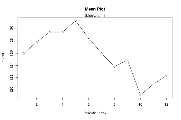
| Title produced by software | Mean Plot | ||||||||||||||||||||
| Date of computation | Fri, 30 Nov 2007 02:56:21 -0700 | ||||||||||||||||||||
| Cite this page as follows | Statistical Computations at FreeStatistics.org, Office for Research Development and Education, URL https://freestatistics.org/blog/index.php?v=date/2007/Nov/30/t1196415951j2xdl69dx6sqefh.htm/, Retrieved Sun, 28 Apr 2024 07:25:12 +0000 | ||||||||||||||||||||
| Statistical Computations at FreeStatistics.org, Office for Research Development and Education, URL https://freestatistics.org/blog/index.php?pk=7626, Retrieved Sun, 28 Apr 2024 07:25:12 +0000 | |||||||||||||||||||||
| QR Codes: | |||||||||||||||||||||
|
| |||||||||||||||||||||
| Original text written by user: | |||||||||||||||||||||
| IsPrivate? | No (this computation is public) | ||||||||||||||||||||
| User-defined keywords | Paper G 29 | ||||||||||||||||||||
| Estimated Impact | 224 | ||||||||||||||||||||
Tree of Dependent Computations | |||||||||||||||||||||
| Family? (F = Feedback message, R = changed R code, M = changed R Module, P = changed Parameters, D = changed Data) | |||||||||||||||||||||
| - [Mean Plot] [Mean Plot Totaal] [2007-11-30 09:56:21] [7a600ca82a81f1b71fd92dcbb183f5b4] [Current] - RMPD [Multiple Regression] [Multiple regressi...] [2007-12-16 23:35:21] [2a62d1c381a3e63644fc037b6df1492b] - RMPD [Multiple Regression] [Multiple regressi...] [2007-12-16 23:41:47] [2a62d1c381a3e63644fc037b6df1492b] | |||||||||||||||||||||
| Feedback Forum | |||||||||||||||||||||
Post a new message | |||||||||||||||||||||
Dataset | |||||||||||||||||||||
| Dataseries X: | |||||||||||||||||||||
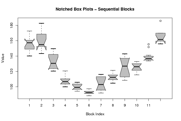
153,4 159,5 157,4 169,1 172,6 161,7 159,2 157,4 153,9 144,8 142,2 140,1 143,4 153,3 166,9 170,6 182,8 170,3 156,6 155,2 154,7 151,6 152,1 153,2 149,5 149,7 144,3 140 137,8 132,2 128,9 123,1 120,4 122,8 126 124,5 120,6 114,7 111,7 109,1 108 107,7 99,9 103,7 103,4 103,4 104,7 105,8 105,3 103 103,8 103,4 105,8 101,4 97 94,3 96,6 97,1 95,7 96,9 97,4 95,3 93,6 91,5 93,1 91,7 94,3 93,9 90,9 88,3 91,3 91,7 92,4 92 95,6 95,8 96,4 99 107 109,7 116,2 115,9 113,8 112,6 113,7 115,9 110,3 111,3 113,4 108,2 104,8 106 110,9 115 118,4 121,4 128,8 131,7 141,7 142,9 139,4 134,7 125 113,6 111,5 108,5 112,3 116,6 115,5 120,1 132,9 128,1 129,3 132,5 131 124,9 120,8 122 122,1 127,4 135,2 137,3 135 136 138,4 134,7 138,4 133,9 133,6 141,2 151,8 155,4 156,6 161,6 160,7 156 159,5 168,7 169,9 169,9 185,9 | |||||||||||||||||||||
Tables (Output of Computation) | |||||||||||||||||||||
| |||||||||||||||||||||
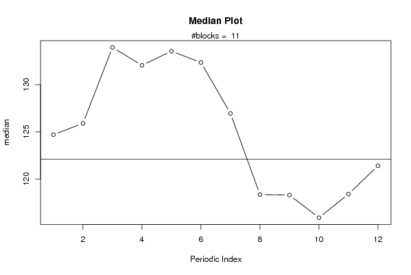
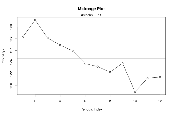
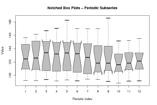
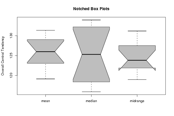
Figures (Output of Computation) | |||||||||||||||||||||
Input Parameters & R Code | |||||||||||||||||||||
| Parameters (Session): | |||||||||||||||||||||
| par1 = 12 ; | |||||||||||||||||||||
| Parameters (R input): | |||||||||||||||||||||
| par1 = 12 ; | |||||||||||||||||||||
| R code (references can be found in the software module): | |||||||||||||||||||||
par1 <- as.numeric(par1) | |||||||||||||||||||||