Repository of Reproducible Computations

Free Statistics

of Irreproducible Research!

Author's title

Author

*Unverified author*

R Software Module

rwasp_autocorrelation.wasp

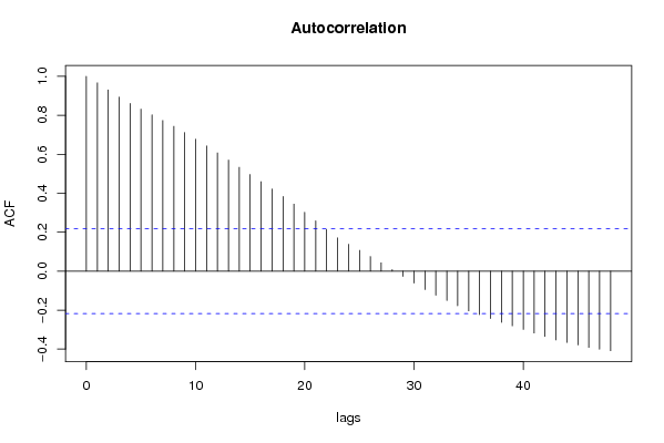
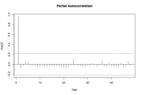
Title produced by software

(Partial) Autocorrelation Function

Date of computation

Wed, 28 Nov 2007 11:26:27 -0700

Cite this page as follows

Statistical Computations at FreeStatistics.org, Office for Research Development and Education, URL https://freestatistics.org/blog/index.php?v=date/2007/Nov/28/t1196273822klusi0u2658kha3.htm/, Retrieved Thu, 02 May 2024 00:37:20 +0000

Statistical Computations at FreeStatistics.org, Office for Research Development and Education, URL https://freestatistics.org/blog/index.php?pk=7198, Retrieved Thu, 02 May 2024 00:37:20 +0000

QR Codes:

Paste this QR Code to cite your computation.

Original text written by user:

IsPrivate?

No (this computation is public)

User-defined keywords

Estimated Impact

199

Family? (F = Feedback message, R = changed R code, M = changed R Module, P = changed Parameters, D = changed Data)

-       [(Partial) Autocorrelation Function] [Autocorrelation -...] [2007-11-28 18:26:27] [bad81931077d8a4f1668ce1551154583] [Current]

Feedback Forum

Post a new message

Dataseries X:

Download CSV

Histogram

Boxplots

4,68
4,68
4,67
4,58
4,48
4,46
4,46
4,46
4,45
4,45
4,45
4,45
4,45
4,45
4,45
4,45
4,44
4,44
4,44
4,44
4,44
4,43
4,38
4,23
4,2
4,2
4,2
4,2
4,2
4,19
4,16
4,06
4
3,99
3,95
3,81
3,8
3,8
3,8
3,8
3,79
3,79
3,78
3,69
3,69
3,69
3,69
3,69
3,69
3,69
3,69
3,68
3,63
3,61
3,61
3,61
3,6
3,58
3,52
3,52
3,52
3,52
3,52
3,52
3,52
3,52
3,52
3,51
3,47
3,43
3,42
3,42
3,42
3,42
3,42
3,42
3,42
3,42
3,42
3,42
3,42

Summary of compuational transaction
Raw Input	view raw input (R code)
Raw Output	view raw output of R engine
Computing time	1 seconds
R Server	'Gwilym Jenkins' @ 72.249.127.135

\begin{tabular}{lllllllll}
\hline
Summary of compuational transaction \tabularnewline
Raw Input & view raw input (R code)  \tabularnewline
Raw Output & view raw output of R engine  \tabularnewline
Computing time & 1 seconds \tabularnewline
R Server & 'Gwilym Jenkins' @ 72.249.127.135 \tabularnewline
\hline
\end{tabular}
%Source: https://freestatistics.org/blog/index.php?pk=7198&T=0

[TABLE]
[ROW][C]Summary of compuational transaction[/C][/ROW]
[ROW][C]Raw Input[/C][C]view raw input (R code) [/C][/ROW]
[ROW][C]Raw Output[/C][C]view raw output of R engine [/C][/ROW]
[ROW][C]Computing time[/C][C]1 seconds[/C][/ROW]
[ROW][C]R Server[/C][C]'Gwilym Jenkins' @ 72.249.127.135[/C][/ROW]
[/TABLE]
Source: https://freestatistics.org/blog/index.php?pk=7198&T=0

Globally Unique Identifier (entire table): ba.freestatistics.org/blog/index.php?pk=7198&T=0

As an alternative you can also use a QR Code:

The GUIDs for individual cells are displayed in the table below:

Summary of compuational transaction
Raw Input	view raw input (R code)
Raw Output	view raw output of R engine
Computing time	1 seconds
R Server	'Gwilym Jenkins' @ 72.249.127.135

Autocorrelation Function
Time lag k	ACF(k)	T-STAT	P-value
0	1	9	0
1	0.967036	8.7033	0
2	0.930664	8.376	0
3	0.893731	8.0436	0
4	0.860569	7.7451	0
5	0.831535	7.4838	0
6	0.802828	7.2254	0
7	0.773522	6.9617	0
8	0.743321	6.6899	0
9	0.711291	6.4016	0
10	0.677518	6.0977	0
11	0.642792	5.7851	0
12	0.606885	5.462	0
13	0.569843	5.1286	1e-06
14	0.533194	4.7987	4e-06
15	0.496481	4.4683	1.3e-05
16	0.459086	4.1318	4.4e-05
17	0.421739	3.7957	0.000142
18	0.383397	3.4506	0.000446
19	0.343882	3.0949	0.001351
20	0.302381	2.7214	0.003977
21	0.258362	2.3253	0.01128
22	0.213675	1.9231	0.028993
23	0.171054	1.5395	0.063791
24	0.137861	1.2408	0.109139
25	0.106631	0.9597	0.170035
26	0.075174	0.6766	0.250304
27	0.042558	0.383	0.351354
28	0.008184	0.0737	0.470733
29	-0.026978	-0.2428	0.595614
30	-0.061085	-0.5498	0.708004
31	-0.094212	-0.8479	0.800506
32	-0.123325	-1.1099	0.864842
33	-0.150364	-1.3533	0.910134
34	-0.177631	-1.5987	0.943107
35	-0.203655	-1.8329	0.964754
36	-0.223207	-2.0089	0.976058
37	-0.242851	-2.1857	0.984136
38	-0.263114	-2.368	0.989867
39	-0.280798	-2.5272	0.993278
40	-0.299014	-2.6911	0.995676
41	-0.317331	-2.856	0.997276
42	-0.335376	-3.0184	0.998302
43	-0.352925	-3.1763	0.998945
44	-0.36564	-3.2908	0.999259
45	-0.378584	-3.4073	0.999488
46	-0.391733	-3.5256	0.999651
47	-0.400508	-3.6046	0.999731

\begin{tabular}{lllllllll}
\hline
Autocorrelation Function \tabularnewline
Time lag k & ACF(k) & T-STAT & P-value \tabularnewline
0 & 1 & 9 & 0 \tabularnewline
1 & 0.967036 & 8.7033 & 0 \tabularnewline
2 & 0.930664 & 8.376 & 0 \tabularnewline
3 & 0.893731 & 8.0436 & 0 \tabularnewline
4 & 0.860569 & 7.7451 & 0 \tabularnewline
5 & 0.831535 & 7.4838 & 0 \tabularnewline
6 & 0.802828 & 7.2254 & 0 \tabularnewline
7 & 0.773522 & 6.9617 & 0 \tabularnewline
8 & 0.743321 & 6.6899 & 0 \tabularnewline
9 & 0.711291 & 6.4016 & 0 \tabularnewline
10 & 0.677518 & 6.0977 & 0 \tabularnewline
11 & 0.642792 & 5.7851 & 0 \tabularnewline
12 & 0.606885 & 5.462 & 0 \tabularnewline
13 & 0.569843 & 5.1286 & 1e-06 \tabularnewline
14 & 0.533194 & 4.7987 & 4e-06 \tabularnewline
15 & 0.496481 & 4.4683 & 1.3e-05 \tabularnewline
16 & 0.459086 & 4.1318 & 4.4e-05 \tabularnewline
17 & 0.421739 & 3.7957 & 0.000142 \tabularnewline
18 & 0.383397 & 3.4506 & 0.000446 \tabularnewline
19 & 0.343882 & 3.0949 & 0.001351 \tabularnewline
20 & 0.302381 & 2.7214 & 0.003977 \tabularnewline
21 & 0.258362 & 2.3253 & 0.01128 \tabularnewline
22 & 0.213675 & 1.9231 & 0.028993 \tabularnewline
23 & 0.171054 & 1.5395 & 0.063791 \tabularnewline
24 & 0.137861 & 1.2408 & 0.109139 \tabularnewline
25 & 0.106631 & 0.9597 & 0.170035 \tabularnewline
26 & 0.075174 & 0.6766 & 0.250304 \tabularnewline
27 & 0.042558 & 0.383 & 0.351354 \tabularnewline
28 & 0.008184 & 0.0737 & 0.470733 \tabularnewline
29 & -0.026978 & -0.2428 & 0.595614 \tabularnewline
30 & -0.061085 & -0.5498 & 0.708004 \tabularnewline
31 & -0.094212 & -0.8479 & 0.800506 \tabularnewline
32 & -0.123325 & -1.1099 & 0.864842 \tabularnewline
33 & -0.150364 & -1.3533 & 0.910134 \tabularnewline
34 & -0.177631 & -1.5987 & 0.943107 \tabularnewline
35 & -0.203655 & -1.8329 & 0.964754 \tabularnewline
36 & -0.223207 & -2.0089 & 0.976058 \tabularnewline
37 & -0.242851 & -2.1857 & 0.984136 \tabularnewline
38 & -0.263114 & -2.368 & 0.989867 \tabularnewline
39 & -0.280798 & -2.5272 & 0.993278 \tabularnewline
40 & -0.299014 & -2.6911 & 0.995676 \tabularnewline
41 & -0.317331 & -2.856 & 0.997276 \tabularnewline
42 & -0.335376 & -3.0184 & 0.998302 \tabularnewline
43 & -0.352925 & -3.1763 & 0.998945 \tabularnewline
44 & -0.36564 & -3.2908 & 0.999259 \tabularnewline
45 & -0.378584 & -3.4073 & 0.999488 \tabularnewline
46 & -0.391733 & -3.5256 & 0.999651 \tabularnewline
47 & -0.400508 & -3.6046 & 0.999731 \tabularnewline
\hline
\end{tabular}
%Source: https://freestatistics.org/blog/index.php?pk=7198&T=1

[TABLE]
[ROW][C]Autocorrelation Function[/C][/ROW]
[ROW][C]Time lag k[/C][C]ACF(k)[/C][C]T-STAT[/C][C]P-value[/C][/ROW]
[ROW][C]0[/C][C]1[/C][C]9[/C][C]0[/C][/ROW]
[ROW][C]1[/C][C]0.967036[/C][C]8.7033[/C][C]0[/C][/ROW]
[ROW][C]2[/C][C]0.930664[/C][C]8.376[/C][C]0[/C][/ROW]
[ROW][C]3[/C][C]0.893731[/C][C]8.0436[/C][C]0[/C][/ROW]
[ROW][C]4[/C][C]0.860569[/C][C]7.7451[/C][C]0[/C][/ROW]
[ROW][C]5[/C][C]0.831535[/C][C]7.4838[/C][C]0[/C][/ROW]
[ROW][C]6[/C][C]0.802828[/C][C]7.2254[/C][C]0[/C][/ROW]
[ROW][C]7[/C][C]0.773522[/C][C]6.9617[/C][C]0[/C][/ROW]
[ROW][C]8[/C][C]0.743321[/C][C]6.6899[/C][C]0[/C][/ROW]
[ROW][C]9[/C][C]0.711291[/C][C]6.4016[/C][C]0[/C][/ROW]
[ROW][C]10[/C][C]0.677518[/C][C]6.0977[/C][C]0[/C][/ROW]
[ROW][C]11[/C][C]0.642792[/C][C]5.7851[/C][C]0[/C][/ROW]
[ROW][C]12[/C][C]0.606885[/C][C]5.462[/C][C]0[/C][/ROW]
[ROW][C]13[/C][C]0.569843[/C][C]5.1286[/C][C]1e-06[/C][/ROW]
[ROW][C]14[/C][C]0.533194[/C][C]4.7987[/C][C]4e-06[/C][/ROW]
[ROW][C]15[/C][C]0.496481[/C][C]4.4683[/C][C]1.3e-05[/C][/ROW]
[ROW][C]16[/C][C]0.459086[/C][C]4.1318[/C][C]4.4e-05[/C][/ROW]
[ROW][C]17[/C][C]0.421739[/C][C]3.7957[/C][C]0.000142[/C][/ROW]
[ROW][C]18[/C][C]0.383397[/C][C]3.4506[/C][C]0.000446[/C][/ROW]
[ROW][C]19[/C][C]0.343882[/C][C]3.0949[/C][C]0.001351[/C][/ROW]
[ROW][C]20[/C][C]0.302381[/C][C]2.7214[/C][C]0.003977[/C][/ROW]
[ROW][C]21[/C][C]0.258362[/C][C]2.3253[/C][C]0.01128[/C][/ROW]
[ROW][C]22[/C][C]0.213675[/C][C]1.9231[/C][C]0.028993[/C][/ROW]
[ROW][C]23[/C][C]0.171054[/C][C]1.5395[/C][C]0.063791[/C][/ROW]
[ROW][C]24[/C][C]0.137861[/C][C]1.2408[/C][C]0.109139[/C][/ROW]
[ROW][C]25[/C][C]0.106631[/C][C]0.9597[/C][C]0.170035[/C][/ROW]
[ROW][C]26[/C][C]0.075174[/C][C]0.6766[/C][C]0.250304[/C][/ROW]
[ROW][C]27[/C][C]0.042558[/C][C]0.383[/C][C]0.351354[/C][/ROW]
[ROW][C]28[/C][C]0.008184[/C][C]0.0737[/C][C]0.470733[/C][/ROW]
[ROW][C]29[/C][C]-0.026978[/C][C]-0.2428[/C][C]0.595614[/C][/ROW]
[ROW][C]30[/C][C]-0.061085[/C][C]-0.5498[/C][C]0.708004[/C][/ROW]
[ROW][C]31[/C][C]-0.094212[/C][C]-0.8479[/C][C]0.800506[/C][/ROW]
[ROW][C]32[/C][C]-0.123325[/C][C]-1.1099[/C][C]0.864842[/C][/ROW]
[ROW][C]33[/C][C]-0.150364[/C][C]-1.3533[/C][C]0.910134[/C][/ROW]
[ROW][C]34[/C][C]-0.177631[/C][C]-1.5987[/C][C]0.943107[/C][/ROW]
[ROW][C]35[/C][C]-0.203655[/C][C]-1.8329[/C][C]0.964754[/C][/ROW]
[ROW][C]36[/C][C]-0.223207[/C][C]-2.0089[/C][C]0.976058[/C][/ROW]
[ROW][C]37[/C][C]-0.242851[/C][C]-2.1857[/C][C]0.984136[/C][/ROW]
[ROW][C]38[/C][C]-0.263114[/C][C]-2.368[/C][C]0.989867[/C][/ROW]
[ROW][C]39[/C][C]-0.280798[/C][C]-2.5272[/C][C]0.993278[/C][/ROW]
[ROW][C]40[/C][C]-0.299014[/C][C]-2.6911[/C][C]0.995676[/C][/ROW]
[ROW][C]41[/C][C]-0.317331[/C][C]-2.856[/C][C]0.997276[/C][/ROW]
[ROW][C]42[/C][C]-0.335376[/C][C]-3.0184[/C][C]0.998302[/C][/ROW]
[ROW][C]43[/C][C]-0.352925[/C][C]-3.1763[/C][C]0.998945[/C][/ROW]
[ROW][C]44[/C][C]-0.36564[/C][C]-3.2908[/C][C]0.999259[/C][/ROW]
[ROW][C]45[/C][C]-0.378584[/C][C]-3.4073[/C][C]0.999488[/C][/ROW]
[ROW][C]46[/C][C]-0.391733[/C][C]-3.5256[/C][C]0.999651[/C][/ROW]
[ROW][C]47[/C][C]-0.400508[/C][C]-3.6046[/C][C]0.999731[/C][/ROW]
[/TABLE]
Source: https://freestatistics.org/blog/index.php?pk=7198&T=1

Globally Unique Identifier (entire table): ba.freestatistics.org/blog/index.php?pk=7198&T=1

As an alternative you can also use a QR Code:

The GUIDs for individual cells are displayed in the table below:

Autocorrelation Function
Time lag k	ACF(k)	T-STAT	P-value
0	1	9	0
1	0.967036	8.7033	0
2	0.930664	8.376	0
3	0.893731	8.0436	0
4	0.860569	7.7451	0
5	0.831535	7.4838	0
6	0.802828	7.2254	0
7	0.773522	6.9617	0
8	0.743321	6.6899	0
9	0.711291	6.4016	0
10	0.677518	6.0977	0
11	0.642792	5.7851	0
12	0.606885	5.462	0
13	0.569843	5.1286	1e-06
14	0.533194	4.7987	4e-06
15	0.496481	4.4683	1.3e-05
16	0.459086	4.1318	4.4e-05
17	0.421739	3.7957	0.000142
18	0.383397	3.4506	0.000446
19	0.343882	3.0949	0.001351
20	0.302381	2.7214	0.003977
21	0.258362	2.3253	0.01128
22	0.213675	1.9231	0.028993
23	0.171054	1.5395	0.063791
24	0.137861	1.2408	0.109139
25	0.106631	0.9597	0.170035
26	0.075174	0.6766	0.250304
27	0.042558	0.383	0.351354
28	0.008184	0.0737	0.470733
29	-0.026978	-0.2428	0.595614
30	-0.061085	-0.5498	0.708004
31	-0.094212	-0.8479	0.800506
32	-0.123325	-1.1099	0.864842
33	-0.150364	-1.3533	0.910134
34	-0.177631	-1.5987	0.943107
35	-0.203655	-1.8329	0.964754
36	-0.223207	-2.0089	0.976058
37	-0.242851	-2.1857	0.984136
38	-0.263114	-2.368	0.989867
39	-0.280798	-2.5272	0.993278
40	-0.299014	-2.6911	0.995676
41	-0.317331	-2.856	0.997276
42	-0.335376	-3.0184	0.998302
43	-0.352925	-3.1763	0.998945
44	-0.36564	-3.2908	0.999259
45	-0.378584	-3.4073	0.999488
46	-0.391733	-3.5256	0.999651
47	-0.400508	-3.6046	0.999731

Partial Autocorrelation Function
Time lag k	PACF(k)	T-STAT	P-value
0	0.967036	8.7033	0
1	-0.069307	-0.6238	0.732731
2	-0.024925	-0.2243	0.588464
3	0.039721	0.3575	0.360829
4	0.04038	0.3634	0.358619
5	-0.018131	-0.1632	0.564607
6	-0.023674	-0.2131	0.584094
7	-0.023161	-0.2085	0.5823
8	-0.040886	-0.368	0.643075
9	-0.043766	-0.3939	0.652653
10	-0.033807	-0.3043	0.619146
11	-0.04143	-0.3729	0.644892
12	-0.043719	-0.3935	0.652496
13	-0.019809	-0.1783	0.570527
14	-0.028503	-0.2565	0.600903
15	-0.039028	-0.3512	0.636843
16	-0.024647	-0.2218	0.587495
17	-0.040208	-0.3619	0.640806
18	-0.045144	-0.4063	0.657203
19	-0.058988	-0.5309	0.701526
20	-0.069125	-0.6221	0.732196
21	-0.045412	-0.4087	0.658085
22	-0.008598	-0.0774	0.530745
23	0.103843	0.9346	0.17639
24	-0.015536	-0.1398	0.555428
25	-0.034033	-0.3063	0.619919
26	-0.026774	-0.241	0.594904
27	-0.035874	-0.3229	0.626186
28	-0.038543	-0.3469	0.635211
29	-0.016521	-0.1487	0.558916
30	-0.023742	-0.2137	0.584331
31	0.019557	0.176	0.430361
32	-0.00951	-0.0856	0.533997
33	-0.040238	-0.3621	0.640904
34	-0.011428	-0.1028	0.540832
35	0.075904	0.6831	0.248234
36	-0.033179	-0.2986	0.616999
37	-0.040674	-0.3661	0.642365
38	0.022289	0.2006	0.420756
39	-0.031214	-0.2809	0.610258
40	-0.042323	-0.3809	0.647865
41	-0.032929	-0.2964	0.616142
42	-0.033042	-0.2974	0.616531
43	0.025092	0.2258	0.410951
44	-0.050035	-0.4503	0.673157
45	-0.03244	-0.292	0.614468
46	0.061527	0.5537	0.29064
47	-0.011079	-0.0997	0.539591

\begin{tabular}{lllllllll}
\hline
Partial Autocorrelation Function \tabularnewline
Time lag k & PACF(k) & T-STAT & P-value \tabularnewline
0 & 0.967036 & 8.7033 & 0 \tabularnewline
1 & -0.069307 & -0.6238 & 0.732731 \tabularnewline
2 & -0.024925 & -0.2243 & 0.588464 \tabularnewline
3 & 0.039721 & 0.3575 & 0.360829 \tabularnewline
4 & 0.04038 & 0.3634 & 0.358619 \tabularnewline
5 & -0.018131 & -0.1632 & 0.564607 \tabularnewline
6 & -0.023674 & -0.2131 & 0.584094 \tabularnewline
7 & -0.023161 & -0.2085 & 0.5823 \tabularnewline
8 & -0.040886 & -0.368 & 0.643075 \tabularnewline
9 & -0.043766 & -0.3939 & 0.652653 \tabularnewline
10 & -0.033807 & -0.3043 & 0.619146 \tabularnewline
11 & -0.04143 & -0.3729 & 0.644892 \tabularnewline
12 & -0.043719 & -0.3935 & 0.652496 \tabularnewline
13 & -0.019809 & -0.1783 & 0.570527 \tabularnewline
14 & -0.028503 & -0.2565 & 0.600903 \tabularnewline
15 & -0.039028 & -0.3512 & 0.636843 \tabularnewline
16 & -0.024647 & -0.2218 & 0.587495 \tabularnewline
17 & -0.040208 & -0.3619 & 0.640806 \tabularnewline
18 & -0.045144 & -0.4063 & 0.657203 \tabularnewline
19 & -0.058988 & -0.5309 & 0.701526 \tabularnewline
20 & -0.069125 & -0.6221 & 0.732196 \tabularnewline
21 & -0.045412 & -0.4087 & 0.658085 \tabularnewline
22 & -0.008598 & -0.0774 & 0.530745 \tabularnewline
23 & 0.103843 & 0.9346 & 0.17639 \tabularnewline
24 & -0.015536 & -0.1398 & 0.555428 \tabularnewline
25 & -0.034033 & -0.3063 & 0.619919 \tabularnewline
26 & -0.026774 & -0.241 & 0.594904 \tabularnewline
27 & -0.035874 & -0.3229 & 0.626186 \tabularnewline
28 & -0.038543 & -0.3469 & 0.635211 \tabularnewline
29 & -0.016521 & -0.1487 & 0.558916 \tabularnewline
30 & -0.023742 & -0.2137 & 0.584331 \tabularnewline
31 & 0.019557 & 0.176 & 0.430361 \tabularnewline
32 & -0.00951 & -0.0856 & 0.533997 \tabularnewline
33 & -0.040238 & -0.3621 & 0.640904 \tabularnewline
34 & -0.011428 & -0.1028 & 0.540832 \tabularnewline
35 & 0.075904 & 0.6831 & 0.248234 \tabularnewline
36 & -0.033179 & -0.2986 & 0.616999 \tabularnewline
37 & -0.040674 & -0.3661 & 0.642365 \tabularnewline
38 & 0.022289 & 0.2006 & 0.420756 \tabularnewline
39 & -0.031214 & -0.2809 & 0.610258 \tabularnewline
40 & -0.042323 & -0.3809 & 0.647865 \tabularnewline
41 & -0.032929 & -0.2964 & 0.616142 \tabularnewline
42 & -0.033042 & -0.2974 & 0.616531 \tabularnewline
43 & 0.025092 & 0.2258 & 0.410951 \tabularnewline
44 & -0.050035 & -0.4503 & 0.673157 \tabularnewline
45 & -0.03244 & -0.292 & 0.614468 \tabularnewline
46 & 0.061527 & 0.5537 & 0.29064 \tabularnewline
47 & -0.011079 & -0.0997 & 0.539591 \tabularnewline
\hline
\end{tabular}
%Source: https://freestatistics.org/blog/index.php?pk=7198&T=2

[TABLE]
[ROW][C]Partial Autocorrelation Function[/C][/ROW]
[ROW][C]Time lag k[/C][C]PACF(k)[/C][C]T-STAT[/C][C]P-value[/C][/ROW]
[ROW][C]0[/C][C]0.967036[/C][C]8.7033[/C][C]0[/C][/ROW]
[ROW][C]1[/C][C]-0.069307[/C][C]-0.6238[/C][C]0.732731[/C][/ROW]
[ROW][C]2[/C][C]-0.024925[/C][C]-0.2243[/C][C]0.588464[/C][/ROW]
[ROW][C]3[/C][C]0.039721[/C][C]0.3575[/C][C]0.360829[/C][/ROW]
[ROW][C]4[/C][C]0.04038[/C][C]0.3634[/C][C]0.358619[/C][/ROW]
[ROW][C]5[/C][C]-0.018131[/C][C]-0.1632[/C][C]0.564607[/C][/ROW]
[ROW][C]6[/C][C]-0.023674[/C][C]-0.2131[/C][C]0.584094[/C][/ROW]
[ROW][C]7[/C][C]-0.023161[/C][C]-0.2085[/C][C]0.5823[/C][/ROW]
[ROW][C]8[/C][C]-0.040886[/C][C]-0.368[/C][C]0.643075[/C][/ROW]
[ROW][C]9[/C][C]-0.043766[/C][C]-0.3939[/C][C]0.652653[/C][/ROW]
[ROW][C]10[/C][C]-0.033807[/C][C]-0.3043[/C][C]0.619146[/C][/ROW]
[ROW][C]11[/C][C]-0.04143[/C][C]-0.3729[/C][C]0.644892[/C][/ROW]
[ROW][C]12[/C][C]-0.043719[/C][C]-0.3935[/C][C]0.652496[/C][/ROW]
[ROW][C]13[/C][C]-0.019809[/C][C]-0.1783[/C][C]0.570527[/C][/ROW]
[ROW][C]14[/C][C]-0.028503[/C][C]-0.2565[/C][C]0.600903[/C][/ROW]
[ROW][C]15[/C][C]-0.039028[/C][C]-0.3512[/C][C]0.636843[/C][/ROW]
[ROW][C]16[/C][C]-0.024647[/C][C]-0.2218[/C][C]0.587495[/C][/ROW]
[ROW][C]17[/C][C]-0.040208[/C][C]-0.3619[/C][C]0.640806[/C][/ROW]
[ROW][C]18[/C][C]-0.045144[/C][C]-0.4063[/C][C]0.657203[/C][/ROW]
[ROW][C]19[/C][C]-0.058988[/C][C]-0.5309[/C][C]0.701526[/C][/ROW]
[ROW][C]20[/C][C]-0.069125[/C][C]-0.6221[/C][C]0.732196[/C][/ROW]
[ROW][C]21[/C][C]-0.045412[/C][C]-0.4087[/C][C]0.658085[/C][/ROW]
[ROW][C]22[/C][C]-0.008598[/C][C]-0.0774[/C][C]0.530745[/C][/ROW]
[ROW][C]23[/C][C]0.103843[/C][C]0.9346[/C][C]0.17639[/C][/ROW]
[ROW][C]24[/C][C]-0.015536[/C][C]-0.1398[/C][C]0.555428[/C][/ROW]
[ROW][C]25[/C][C]-0.034033[/C][C]-0.3063[/C][C]0.619919[/C][/ROW]
[ROW][C]26[/C][C]-0.026774[/C][C]-0.241[/C][C]0.594904[/C][/ROW]
[ROW][C]27[/C][C]-0.035874[/C][C]-0.3229[/C][C]0.626186[/C][/ROW]
[ROW][C]28[/C][C]-0.038543[/C][C]-0.3469[/C][C]0.635211[/C][/ROW]
[ROW][C]29[/C][C]-0.016521[/C][C]-0.1487[/C][C]0.558916[/C][/ROW]
[ROW][C]30[/C][C]-0.023742[/C][C]-0.2137[/C][C]0.584331[/C][/ROW]
[ROW][C]31[/C][C]0.019557[/C][C]0.176[/C][C]0.430361[/C][/ROW]
[ROW][C]32[/C][C]-0.00951[/C][C]-0.0856[/C][C]0.533997[/C][/ROW]
[ROW][C]33[/C][C]-0.040238[/C][C]-0.3621[/C][C]0.640904[/C][/ROW]
[ROW][C]34[/C][C]-0.011428[/C][C]-0.1028[/C][C]0.540832[/C][/ROW]
[ROW][C]35[/C][C]0.075904[/C][C]0.6831[/C][C]0.248234[/C][/ROW]
[ROW][C]36[/C][C]-0.033179[/C][C]-0.2986[/C][C]0.616999[/C][/ROW]
[ROW][C]37[/C][C]-0.040674[/C][C]-0.3661[/C][C]0.642365[/C][/ROW]
[ROW][C]38[/C][C]0.022289[/C][C]0.2006[/C][C]0.420756[/C][/ROW]
[ROW][C]39[/C][C]-0.031214[/C][C]-0.2809[/C][C]0.610258[/C][/ROW]
[ROW][C]40[/C][C]-0.042323[/C][C]-0.3809[/C][C]0.647865[/C][/ROW]
[ROW][C]41[/C][C]-0.032929[/C][C]-0.2964[/C][C]0.616142[/C][/ROW]
[ROW][C]42[/C][C]-0.033042[/C][C]-0.2974[/C][C]0.616531[/C][/ROW]
[ROW][C]43[/C][C]0.025092[/C][C]0.2258[/C][C]0.410951[/C][/ROW]
[ROW][C]44[/C][C]-0.050035[/C][C]-0.4503[/C][C]0.673157[/C][/ROW]
[ROW][C]45[/C][C]-0.03244[/C][C]-0.292[/C][C]0.614468[/C][/ROW]
[ROW][C]46[/C][C]0.061527[/C][C]0.5537[/C][C]0.29064[/C][/ROW]
[ROW][C]47[/C][C]-0.011079[/C][C]-0.0997[/C][C]0.539591[/C][/ROW]
[/TABLE]
Source: https://freestatistics.org/blog/index.php?pk=7198&T=2

Globally Unique Identifier (entire table): ba.freestatistics.org/blog/index.php?pk=7198&T=2

As an alternative you can also use a QR Code:

The GUIDs for individual cells are displayed in the table below:

Partial Autocorrelation Function
Time lag k	PACF(k)	T-STAT	P-value
0	0.967036	8.7033	0
1	-0.069307	-0.6238	0.732731
2	-0.024925	-0.2243	0.588464
3	0.039721	0.3575	0.360829
4	0.04038	0.3634	0.358619
5	-0.018131	-0.1632	0.564607
6	-0.023674	-0.2131	0.584094
7	-0.023161	-0.2085	0.5823
8	-0.040886	-0.368	0.643075
9	-0.043766	-0.3939	0.652653
10	-0.033807	-0.3043	0.619146
11	-0.04143	-0.3729	0.644892
12	-0.043719	-0.3935	0.652496
13	-0.019809	-0.1783	0.570527
14	-0.028503	-0.2565	0.600903
15	-0.039028	-0.3512	0.636843
16	-0.024647	-0.2218	0.587495
17	-0.040208	-0.3619	0.640806
18	-0.045144	-0.4063	0.657203
19	-0.058988	-0.5309	0.701526
20	-0.069125	-0.6221	0.732196
21	-0.045412	-0.4087	0.658085
22	-0.008598	-0.0774	0.530745
23	0.103843	0.9346	0.17639
24	-0.015536	-0.1398	0.555428
25	-0.034033	-0.3063	0.619919
26	-0.026774	-0.241	0.594904
27	-0.035874	-0.3229	0.626186
28	-0.038543	-0.3469	0.635211
29	-0.016521	-0.1487	0.558916
30	-0.023742	-0.2137	0.584331
31	0.019557	0.176	0.430361
32	-0.00951	-0.0856	0.533997
33	-0.040238	-0.3621	0.640904
34	-0.011428	-0.1028	0.540832
35	0.075904	0.6831	0.248234
36	-0.033179	-0.2986	0.616999
37	-0.040674	-0.3661	0.642365
38	0.022289	0.2006	0.420756
39	-0.031214	-0.2809	0.610258
40	-0.042323	-0.3809	0.647865
41	-0.032929	-0.2964	0.616142
42	-0.033042	-0.2974	0.616531
43	0.025092	0.2258	0.410951
44	-0.050035	-0.4503	0.673157
45	-0.03244	-0.292	0.614468
46	0.061527	0.5537	0.29064
47	-0.011079	-0.0997	0.539591

Figure 1

PNG link

Postscript link

PDF link

Figure 2

PNG link

Postscript link

PDF link

Parameters (Session):

par1 = 12 ;

Parameters (R input):

par1 = 48 ; par2 = 1 ; par3 = 0 ; par4 = 0 ; par5 = 12 ;

R code (references can be found in the software module):

if (par1 == 'Default') {
par1 = 10*log10(length(x))
} else {
par1 <- as.numeric(par1)
}
par2 <- as.numeric(par2)
par3 <- as.numeric(par3)
par4 <- as.numeric(par4)
par5 <- as.numeric(par5)
if (par2 == 0) {
x <- log(x)
} else {
x <- (x ^ par2 - 1) / par2
}
if (par3 > 0) x <- diff(x,lag=1,difference=par3)
if (par4 > 0) x <- diff(x,lag=par5,difference=par4)
bitmap(file='pic1.png')
racf <- acf(x,par1,main='Autocorrelation',xlab='lags',ylab='ACF')
dev.off()
bitmap(file='pic2.png')
rpacf <- pacf(x,par1,main='Partial Autocorrelation',xlab='lags',ylab='PACF')
dev.off()
(myacf <- c(racf$acf))
(mypacf <- c(rpacf$acf))
lengthx <- length(x)
sqrtn <- sqrt(lengthx)
load(file='createtable')
a<-table.start()
a<-table.row.start(a)
a<-table.element(a,'Autocorrelation Function',4,TRUE)
a<-table.row.end(a)
a<-table.row.start(a)
a<-table.element(a,'Time lag k',header=TRUE)
a<-table.element(a,hyperlink('basics.htm','ACF(k)','click here for more information about the Autocorrelation Function'),header=TRUE)
a<-table.element(a,'T-STAT',header=TRUE)
a<-table.element(a,'P-value',header=TRUE)
a<-table.row.end(a)
for (i in 1:par1) {
a<-table.row.start(a)
a<-table.element(a,i-1,header=TRUE)
a<-table.element(a,round(myacf[i],6))
mytstat <- myacf[i]*sqrtn
a<-table.element(a,round(mytstat,4))
a<-table.element(a,round(1-pt(mytstat,lengthx),6))
a<-table.row.end(a)
}
a<-table.end(a)
table.save(a,file='mytable.tab')
a<-table.start()
a<-table.row.start(a)
a<-table.element(a,'Partial Autocorrelation Function',4,TRUE)
a<-table.row.end(a)
a<-table.row.start(a)
a<-table.element(a,'Time lag k',header=TRUE)
a<-table.element(a,hyperlink('basics.htm','PACF(k)','click here for more information about the Partial Autocorrelation Function'),header=TRUE)
a<-table.element(a,'T-STAT',header=TRUE)
a<-table.element(a,'P-value',header=TRUE)
a<-table.row.end(a)
for (i in 1:par1) {
a<-table.row.start(a)
a<-table.element(a,i-1,header=TRUE)
a<-table.element(a,round(mypacf[i],6))
mytstat <- mypacf[i]*sqrtn
a<-table.element(a,round(mytstat,4))
a<-table.element(a,round(1-pt(mytstat,lengthx),6))
a<-table.row.end(a)
}
a<-table.end(a)
table.save(a,file='mytable1.tab')

Free Statistics

Description of Statistical Computation

Tree of Dependent Computations

Dataset

Tables (Output of Computation)

Figures (Output of Computation)

Input Parameters & R Code