Repository of Reproducible Computations

Free Statistics

of Irreproducible Research!

Author's title

Author

*Unverified author*

R Software Module

rwasp_spectrum.wasp

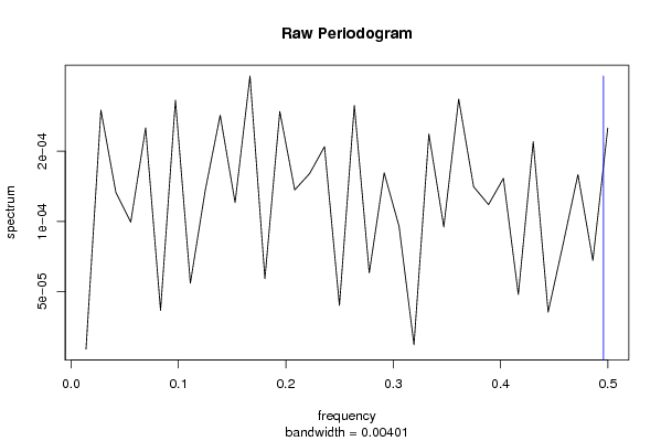
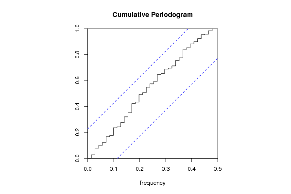
Title produced by software

Spectral Analysis

Date of computation

Wed, 28 Nov 2007 04:45:43 -0700

Cite this page as follows

Statistical Computations at FreeStatistics.org, Office for Research Development and Education, URL https://freestatistics.org/blog/index.php?v=date/2007/Nov/28/t1196249721lkock7l85hhmgbt.htm/, Retrieved Thu, 02 May 2024 01:10:28 +0000

Statistical Computations at FreeStatistics.org, Office for Research Development and Education, URL https://freestatistics.org/blog/index.php?pk=7032, Retrieved Thu, 02 May 2024 01:10:28 +0000

QR Codes:

Paste this QR Code to cite your computation.

Original text written by user:

IsPrivate?

No (this computation is public)

User-defined keywords

Estimated Impact

203

Family? (F = Feedback message, R = changed R code, M = changed R Module, P = changed Parameters, D = changed Data)

-       [Spectral Analysis] [Inducing Stationa...] [2007-11-28 11:45:43] [157a0cf3c12a7482b4e6935b4c49d48f] [Current]

Feedback Forum

Post a new message

Dataseries X:

Download CSV

Histogram

Boxplots

1,43
1,43
1,43
1,43
1,43
1,43
1,43
1,43
1,43
1,43
1,43
1,43
1,43
1,43
1,43
1,43
1,43
1,43
1,44
1,48
1,48
1,48
1,48
1,48
1,48
1,48
1,48
1,48
1,48
1,48
1,48
1,48
1,48
1,48
1,48
1,48
1,48
1,48
1,48
1,48
1,48
1,48
1,48
1,48
1,48
1,48
1,48
1,48
1,48
1,57
1,58
1.58
1,58
1,58
1,59
1,6
1,6
1,61
1,61
1,61
1,62
1,63
1,63
1,64
1,64
1,64
1,64
1,64
1,65
1,65
1,65
1,65

Summary of compuational transaction
Raw Input	view raw input (R code)
Raw Output	view raw output of R engine
Computing time	2 seconds
R Server	'Gwilym Jenkins' @ 72.249.127.135

\begin{tabular}{lllllllll}
\hline
Summary of compuational transaction \tabularnewline
Raw Input & view raw input (R code)  \tabularnewline
Raw Output & view raw output of R engine  \tabularnewline
Computing time & 2 seconds \tabularnewline
R Server & 'Gwilym Jenkins' @ 72.249.127.135 \tabularnewline
\hline
\end{tabular}
%Source: https://freestatistics.org/blog/index.php?pk=7032&T=0

[TABLE]
[ROW][C]Summary of compuational transaction[/C][/ROW]
[ROW][C]Raw Input[/C][C]view raw input (R code) [/C][/ROW]
[ROW][C]Raw Output[/C][C]view raw output of R engine [/C][/ROW]
[ROW][C]Computing time[/C][C]2 seconds[/C][/ROW]
[ROW][C]R Server[/C][C]'Gwilym Jenkins' @ 72.249.127.135[/C][/ROW]
[/TABLE]
Source: https://freestatistics.org/blog/index.php?pk=7032&T=0

Globally Unique Identifier (entire table): ba.freestatistics.org/blog/index.php?pk=7032&T=0

As an alternative you can also use a QR Code:

The GUIDs for individual cells are displayed in the table below:

Summary of compuational transaction
Raw Input	view raw input (R code)
Raw Output	view raw output of R engine
Computing time	2 seconds
R Server	'Gwilym Jenkins' @ 72.249.127.135

Raw Periodogram
Parameter	Value
Box-Cox transformation parameter (lambda)	1
Degree of non-seasonal differencing (d)	1
Degree of seasonal differencing (D)	0
Seasonal Period (s)	3
Frequency (Period)	Spectrum
0.0139 (72)	2.8e-05
0.0278 (36)	3e-04
0.0417 (24)	0.000133
0.0556 (18)	9.9e-05
0.0694 (14.4)	0.000252
0.0833 (12)	4.2e-05
0.0972 (10.2857)	0.000331
0.1111 (9)	5.4e-05
0.125 (8)	0.000136
0.1389 (7.2)	0.000285
0.1528 (6.5455)	0.00012
0.1667 (6)	0.00042
0.1806 (5.5385)	5.7e-05
0.1944 (5.1429)	0.000296
0.2083 (4.8)	0.000136
0.2222 (4.5)	0.00016
0.2361 (4.2353)	0.000209
0.25 (4)	4.4e-05
0.2639 (3.7895)	0.000315
0.2778 (3.6)	6e-05
0.2917 (3.4286)	0.000162
0.3056 (3.2727)	9.5e-05
0.3194 (3.1304)	3e-05
0.3333 (3)	0.000237
0.3472 (2.88)	9.5e-05
0.3611 (2.7692)	0.000335
0.375 (2.6667)	0.000141
0.3889 (2.5714)	0.000118
0.4028 (2.4828)	0.000153
0.4167 (2.4)	4.9e-05
0.4306 (2.3226)	0.00022
0.4444 (2.25)	4.1e-05
0.4583 (2.1818)	8e-05
0.4722 (2.1176)	0.000159
0.4861 (2.0571)	6.8e-05
0.5 (2)	0.000252

\begin{tabular}{lllllllll}
\hline
Raw Periodogram \tabularnewline
Parameter & Value \tabularnewline
Box-Cox transformation parameter (lambda) & 1 \tabularnewline
Degree of non-seasonal differencing (d) & 1 \tabularnewline
Degree of seasonal differencing (D) & 0 \tabularnewline
Seasonal Period (s) & 3 \tabularnewline
Frequency (Period) & Spectrum \tabularnewline
0.0139 (72) & 2.8e-05 \tabularnewline
0.0278 (36) & 3e-04 \tabularnewline
0.0417 (24) & 0.000133 \tabularnewline
0.0556 (18) & 9.9e-05 \tabularnewline
0.0694 (14.4) & 0.000252 \tabularnewline
0.0833 (12) & 4.2e-05 \tabularnewline
0.0972 (10.2857) & 0.000331 \tabularnewline
0.1111 (9) & 5.4e-05 \tabularnewline
0.125 (8) & 0.000136 \tabularnewline
0.1389 (7.2) & 0.000285 \tabularnewline
0.1528 (6.5455) & 0.00012 \tabularnewline
0.1667 (6) & 0.00042 \tabularnewline
0.1806 (5.5385) & 5.7e-05 \tabularnewline
0.1944 (5.1429) & 0.000296 \tabularnewline
0.2083 (4.8) & 0.000136 \tabularnewline
0.2222 (4.5) & 0.00016 \tabularnewline
0.2361 (4.2353) & 0.000209 \tabularnewline
0.25 (4) & 4.4e-05 \tabularnewline
0.2639 (3.7895) & 0.000315 \tabularnewline
0.2778 (3.6) & 6e-05 \tabularnewline
0.2917 (3.4286) & 0.000162 \tabularnewline
0.3056 (3.2727) & 9.5e-05 \tabularnewline
0.3194 (3.1304) & 3e-05 \tabularnewline
0.3333 (3) & 0.000237 \tabularnewline
0.3472 (2.88) & 9.5e-05 \tabularnewline
0.3611 (2.7692) & 0.000335 \tabularnewline
0.375 (2.6667) & 0.000141 \tabularnewline
0.3889 (2.5714) & 0.000118 \tabularnewline
0.4028 (2.4828) & 0.000153 \tabularnewline
0.4167 (2.4) & 4.9e-05 \tabularnewline
0.4306 (2.3226) & 0.00022 \tabularnewline
0.4444 (2.25) & 4.1e-05 \tabularnewline
0.4583 (2.1818) & 8e-05 \tabularnewline
0.4722 (2.1176) & 0.000159 \tabularnewline
0.4861 (2.0571) & 6.8e-05 \tabularnewline
0.5 (2) & 0.000252 \tabularnewline
\hline
\end{tabular}
%Source: https://freestatistics.org/blog/index.php?pk=7032&T=1

[TABLE]
[ROW][C]Raw Periodogram[/C][/ROW]
[ROW][C]Parameter[/C][C]Value[/C][/ROW]
[ROW][C]Box-Cox transformation parameter (lambda)[/C][C]1[/C][/ROW]
[ROW][C]Degree of non-seasonal differencing (d)[/C][C]1[/C][/ROW]
[ROW][C]Degree of seasonal differencing (D)[/C][C]0[/C][/ROW]
[ROW][C]Seasonal Period (s)[/C][C]3[/C][/ROW]
[ROW][C]Frequency (Period)[/C][C]Spectrum[/C][/ROW]
[ROW][C]0.0139 (72)[/C][C]2.8e-05[/C][/ROW]
[ROW][C]0.0278 (36)[/C][C]3e-04[/C][/ROW]
[ROW][C]0.0417 (24)[/C][C]0.000133[/C][/ROW]
[ROW][C]0.0556 (18)[/C][C]9.9e-05[/C][/ROW]
[ROW][C]0.0694 (14.4)[/C][C]0.000252[/C][/ROW]
[ROW][C]0.0833 (12)[/C][C]4.2e-05[/C][/ROW]
[ROW][C]0.0972 (10.2857)[/C][C]0.000331[/C][/ROW]
[ROW][C]0.1111 (9)[/C][C]5.4e-05[/C][/ROW]
[ROW][C]0.125 (8)[/C][C]0.000136[/C][/ROW]
[ROW][C]0.1389 (7.2)[/C][C]0.000285[/C][/ROW]
[ROW][C]0.1528 (6.5455)[/C][C]0.00012[/C][/ROW]
[ROW][C]0.1667 (6)[/C][C]0.00042[/C][/ROW]
[ROW][C]0.1806 (5.5385)[/C][C]5.7e-05[/C][/ROW]
[ROW][C]0.1944 (5.1429)[/C][C]0.000296[/C][/ROW]
[ROW][C]0.2083 (4.8)[/C][C]0.000136[/C][/ROW]
[ROW][C]0.2222 (4.5)[/C][C]0.00016[/C][/ROW]
[ROW][C]0.2361 (4.2353)[/C][C]0.000209[/C][/ROW]
[ROW][C]0.25 (4)[/C][C]4.4e-05[/C][/ROW]
[ROW][C]0.2639 (3.7895)[/C][C]0.000315[/C][/ROW]
[ROW][C]0.2778 (3.6)[/C][C]6e-05[/C][/ROW]
[ROW][C]0.2917 (3.4286)[/C][C]0.000162[/C][/ROW]
[ROW][C]0.3056 (3.2727)[/C][C]9.5e-05[/C][/ROW]
[ROW][C]0.3194 (3.1304)[/C][C]3e-05[/C][/ROW]
[ROW][C]0.3333 (3)[/C][C]0.000237[/C][/ROW]
[ROW][C]0.3472 (2.88)[/C][C]9.5e-05[/C][/ROW]
[ROW][C]0.3611 (2.7692)[/C][C]0.000335[/C][/ROW]
[ROW][C]0.375 (2.6667)[/C][C]0.000141[/C][/ROW]
[ROW][C]0.3889 (2.5714)[/C][C]0.000118[/C][/ROW]
[ROW][C]0.4028 (2.4828)[/C][C]0.000153[/C][/ROW]
[ROW][C]0.4167 (2.4)[/C][C]4.9e-05[/C][/ROW]
[ROW][C]0.4306 (2.3226)[/C][C]0.00022[/C][/ROW]
[ROW][C]0.4444 (2.25)[/C][C]4.1e-05[/C][/ROW]
[ROW][C]0.4583 (2.1818)[/C][C]8e-05[/C][/ROW]
[ROW][C]0.4722 (2.1176)[/C][C]0.000159[/C][/ROW]
[ROW][C]0.4861 (2.0571)[/C][C]6.8e-05[/C][/ROW]
[ROW][C]0.5 (2)[/C][C]0.000252[/C][/ROW]
[/TABLE]
Source: https://freestatistics.org/blog/index.php?pk=7032&T=1

Globally Unique Identifier (entire table): ba.freestatistics.org/blog/index.php?pk=7032&T=1

As an alternative you can also use a QR Code:

The GUIDs for individual cells are displayed in the table below:

Raw Periodogram
Parameter	Value
Box-Cox transformation parameter (lambda)	1
Degree of non-seasonal differencing (d)	1
Degree of seasonal differencing (D)	0
Seasonal Period (s)	3
Frequency (Period)	Spectrum
0.0139 (72)	2.8e-05
0.0278 (36)	3e-04
0.0417 (24)	0.000133
0.0556 (18)	9.9e-05
0.0694 (14.4)	0.000252
0.0833 (12)	4.2e-05
0.0972 (10.2857)	0.000331
0.1111 (9)	5.4e-05
0.125 (8)	0.000136
0.1389 (7.2)	0.000285
0.1528 (6.5455)	0.00012
0.1667 (6)	0.00042
0.1806 (5.5385)	5.7e-05
0.1944 (5.1429)	0.000296
0.2083 (4.8)	0.000136
0.2222 (4.5)	0.00016
0.2361 (4.2353)	0.000209
0.25 (4)	4.4e-05
0.2639 (3.7895)	0.000315
0.2778 (3.6)	6e-05
0.2917 (3.4286)	0.000162
0.3056 (3.2727)	9.5e-05
0.3194 (3.1304)	3e-05
0.3333 (3)	0.000237
0.3472 (2.88)	9.5e-05
0.3611 (2.7692)	0.000335
0.375 (2.6667)	0.000141
0.3889 (2.5714)	0.000118
0.4028 (2.4828)	0.000153
0.4167 (2.4)	4.9e-05
0.4306 (2.3226)	0.00022
0.4444 (2.25)	4.1e-05
0.4583 (2.1818)	8e-05
0.4722 (2.1176)	0.000159
0.4861 (2.0571)	6.8e-05
0.5 (2)	0.000252

Figure 1

PNG link

Postscript link

PDF link

Figure 2

PNG link

Postscript link

PDF link

Parameters (Session):

par1 = Default ; par2 = 1 ; par3 = 1 ; par4 = 1 ; par5 = 12 ;

Parameters (R input):

par1 = 1 ; par2 = 1 ; par3 = 0 ; par4 = 3 ;

R code (references can be found in the software module):

par1 <- as.numeric(par1)
par2 <- as.numeric(par2)
par3 <- as.numeric(par3)
par4 <- as.numeric(par4)
if (par1 == 0) {
x <- log(x)
} else {
x <- (x ^ par1 - 1) / par1
}
if (par2 > 0) x <- diff(x,lag=1,difference=par2)
if (par3 > 0) x <- diff(x,lag=par4,difference=par3)
bitmap(file='test1.png')
r <- spectrum(x,main='Raw Periodogram')
dev.off()
bitmap(file='test2.png')
cpgram(x,main='Cumulative Periodogram')
dev.off()
load(file='createtable')
a<-table.start()
a<-table.row.start(a)
a<-table.element(a,'Raw Periodogram',2,TRUE)
a<-table.row.end(a)
a<-table.row.start(a)
a<-table.element(a,'Parameter',header=TRUE)
a<-table.element(a,'Value',header=TRUE)
a<-table.row.end(a)
a<-table.row.start(a)
a<-table.element(a,'Box-Cox transformation parameter (lambda)',header=TRUE)
a<-table.element(a,par1)
a<-table.row.end(a)
a<-table.row.start(a)
a<-table.element(a,'Degree of non-seasonal differencing (d)',header=TRUE)
a<-table.element(a,par2)
a<-table.row.end(a)
a<-table.row.start(a)
a<-table.element(a,'Degree of seasonal differencing (D)',header=TRUE)
a<-table.element(a,par3)
a<-table.row.end(a)
a<-table.row.start(a)
a<-table.element(a,'Seasonal Period (s)',header=TRUE)
a<-table.element(a,par4)
a<-table.row.end(a)
a<-table.row.start(a)
a<-table.element(a,'Frequency (Period)',header=TRUE)
a<-table.element(a,'Spectrum',header=TRUE)
a<-table.row.end(a)
for (i in 1:length(r$freq)) {
a<-table.row.start(a)
mylab <- round(r$freq[i],4)
mylab <- paste(mylab,' (',sep='')
mylab <- paste(mylab,round(1/r$freq[i],4),sep='')
mylab <- paste(mylab,')',sep='')
a<-table.element(a,mylab,header=TRUE)
a<-table.element(a,round(r$spec[i],6))
a<-table.row.end(a)
}
a<-table.end(a)
table.save(a,file='mytable.tab')

Free Statistics

Description of Statistical Computation

Tree of Dependent Computations

Dataset

Tables (Output of Computation)

Figures (Output of Computation)

Input Parameters & R Code