Repository of Reproducible Computations

Free Statistics

of Irreproducible Research!

Author's title

Author

*Unverified author*

R Software Module

rwasp_autocorrelation.wasp

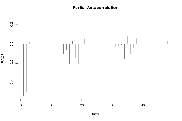
Title produced by software

(Partial) Autocorrelation Function

Date of computation

Tue, 27 Nov 2007 06:16:31 -0700

Cite this page as follows

Statistical Computations at FreeStatistics.org, Office for Research Development and Education, URL https://freestatistics.org/blog/index.php?v=date/2007/Nov/27/t1196168819r1dpj2e4vp5mj7z.htm/, Retrieved Sun, 05 May 2024 18:47:10 +0000

Statistical Computations at FreeStatistics.org, Office for Research Development and Education, URL https://freestatistics.org/blog/index.php?pk=6867, Retrieved Sun, 05 May 2024 18:47:10 +0000

QR Codes:

Paste this QR Code to cite your computation.

Original text written by user:

d=1 D=1

IsPrivate?

No (this computation is public)

User-defined keywords

Q2, reeks 3

Estimated Impact

172

Family? (F = Feedback message, R = changed R code, M = changed R Module, P = changed Parameters, D = changed Data)

-       [(Partial) Autocorrelation Function] [Workshop 3 Q2] [2007-11-27 13:16:31] [e38ae300fa323c405e42b78372d772d6] [Current]

Feedback Forum

Post a new message

Dataseries X:

Download CSV

Histogram

Boxplots

Summary of compuational transaction
Raw Input	view raw input (R code)
Raw Output	view raw output of R engine
Computing time	2 seconds
R Server	'Gwilym Jenkins' @ 72.249.127.135

\begin{tabular}{lllllllll}
\hline
Summary of compuational transaction \tabularnewline
Raw Input & view raw input (R code)  \tabularnewline
Raw Output & view raw output of R engine  \tabularnewline
Computing time & 2 seconds \tabularnewline
R Server & 'Gwilym Jenkins' @ 72.249.127.135 \tabularnewline
\hline
\end{tabular}
%Source: https://freestatistics.org/blog/index.php?pk=6867&T=0

[TABLE]
[ROW][C]Summary of compuational transaction[/C][/ROW]
[ROW][C]Raw Input[/C][C]view raw input (R code) [/C][/ROW]
[ROW][C]Raw Output[/C][C]view raw output of R engine [/C][/ROW]
[ROW][C]Computing time[/C][C]2 seconds[/C][/ROW]
[ROW][C]R Server[/C][C]'Gwilym Jenkins' @ 72.249.127.135[/C][/ROW]
[/TABLE]
Source: https://freestatistics.org/blog/index.php?pk=6867&T=0

Globally Unique Identifier (entire table): ba.freestatistics.org/blog/index.php?pk=6867&T=0

As an alternative you can also use a QR Code:

The GUIDs for individual cells are displayed in the table below:

Summary of compuational transaction
Raw Input	view raw input (R code)
Raw Output	view raw output of R engine
Computing time	2 seconds
R Server	'Gwilym Jenkins' @ 72.249.127.135

Autocorrelation Function
Time lag k	ACF(k)	T-STAT	P-value
0	1	8.2462	0
1	-0.533021	-4.3954	0.99998
2	-0.067427	-0.556	0.709989
3	0.323795	2.6701	0.004739
4	-0.229537	-1.8928	0.96868
5	-0.105033	-0.8661	0.805266
6	0.274587	2.2643	0.013374
7	-0.230303	-1.8991	0.969104
8	0.152575	1.2582	0.106317
9	-0.029794	-0.2457	0.59667
10	-0.126572	-1.0437	0.849848
11	0.210506	1.7359	0.043558
12	-0.216567	-1.7859	0.960709
13	0.063813	0.5262	0.300224
14	0.086307	0.7117	0.23954
15	-0.125699	-1.0365	0.848189
16	-0.030187	-0.2489	0.597918
17	0.232768	1.9195	0.029562
18	-0.31397	-2.5891	0.99412
19	0.137074	1.1303	0.131151
20	0.119631	0.9865	0.163692
21	-0.1505	-1.2411	0.890576
22	-0.00411	-0.0339	0.51347
23	0.226992	1.8718	0.032766
24	-0.273348	-2.2541	0.986291
25	0.03637	0.2999	0.38258
26	0.126077	1.0397	0.151091
27	-0.094081	-0.7758	0.779724
28	0.000389	0.0032	0.498726
29	0.096069	0.7922	0.215498
30	-0.062249	-0.5133	0.695304
31	0.017827	0.147	0.441782
32	-0.019708	-0.1625	0.564308
33	-0.010015	-0.0826	0.532788
34	0.029658	0.2446	0.403766
35	-0.006286	-0.0518	0.520595
36	-0.046726	-0.3853	0.649397
37	0.109672	0.9044	0.184494
38	-0.053043	-0.4374	0.668397
39	-0.055518	-0.4578	0.675727
40	0.120143	0.9907	0.162667
41	-0.140151	-1.1557	0.874079
42	0.028796	0.2375	0.406507
43	0.142488	1.175	0.12205
44	-0.195826	-1.6148	0.94451
45	0.085164	0.7023	0.24245
46	0.067424	0.556	0.290021
47	-0.175346	-1.4459	0.923606

\begin{tabular}{lllllllll}
\hline
Autocorrelation Function \tabularnewline
Time lag k & ACF(k) & T-STAT & P-value \tabularnewline
0 & 1 & 8.2462 & 0 \tabularnewline
1 & -0.533021 & -4.3954 & 0.99998 \tabularnewline
2 & -0.067427 & -0.556 & 0.709989 \tabularnewline
3 & 0.323795 & 2.6701 & 0.004739 \tabularnewline
4 & -0.229537 & -1.8928 & 0.96868 \tabularnewline
5 & -0.105033 & -0.8661 & 0.805266 \tabularnewline
6 & 0.274587 & 2.2643 & 0.013374 \tabularnewline
7 & -0.230303 & -1.8991 & 0.969104 \tabularnewline
8 & 0.152575 & 1.2582 & 0.106317 \tabularnewline
9 & -0.029794 & -0.2457 & 0.59667 \tabularnewline
10 & -0.126572 & -1.0437 & 0.849848 \tabularnewline
11 & 0.210506 & 1.7359 & 0.043558 \tabularnewline
12 & -0.216567 & -1.7859 & 0.960709 \tabularnewline
13 & 0.063813 & 0.5262 & 0.300224 \tabularnewline
14 & 0.086307 & 0.7117 & 0.23954 \tabularnewline
15 & -0.125699 & -1.0365 & 0.848189 \tabularnewline
16 & -0.030187 & -0.2489 & 0.597918 \tabularnewline
17 & 0.232768 & 1.9195 & 0.029562 \tabularnewline
18 & -0.31397 & -2.5891 & 0.99412 \tabularnewline
19 & 0.137074 & 1.1303 & 0.131151 \tabularnewline
20 & 0.119631 & 0.9865 & 0.163692 \tabularnewline
21 & -0.1505 & -1.2411 & 0.890576 \tabularnewline
22 & -0.00411 & -0.0339 & 0.51347 \tabularnewline
23 & 0.226992 & 1.8718 & 0.032766 \tabularnewline
24 & -0.273348 & -2.2541 & 0.986291 \tabularnewline
25 & 0.03637 & 0.2999 & 0.38258 \tabularnewline
26 & 0.126077 & 1.0397 & 0.151091 \tabularnewline
27 & -0.094081 & -0.7758 & 0.779724 \tabularnewline
28 & 0.000389 & 0.0032 & 0.498726 \tabularnewline
29 & 0.096069 & 0.7922 & 0.215498 \tabularnewline
30 & -0.062249 & -0.5133 & 0.695304 \tabularnewline
31 & 0.017827 & 0.147 & 0.441782 \tabularnewline
32 & -0.019708 & -0.1625 & 0.564308 \tabularnewline
33 & -0.010015 & -0.0826 & 0.532788 \tabularnewline
34 & 0.029658 & 0.2446 & 0.403766 \tabularnewline
35 & -0.006286 & -0.0518 & 0.520595 \tabularnewline
36 & -0.046726 & -0.3853 & 0.649397 \tabularnewline
37 & 0.109672 & 0.9044 & 0.184494 \tabularnewline
38 & -0.053043 & -0.4374 & 0.668397 \tabularnewline
39 & -0.055518 & -0.4578 & 0.675727 \tabularnewline
40 & 0.120143 & 0.9907 & 0.162667 \tabularnewline
41 & -0.140151 & -1.1557 & 0.874079 \tabularnewline
42 & 0.028796 & 0.2375 & 0.406507 \tabularnewline
43 & 0.142488 & 1.175 & 0.12205 \tabularnewline
44 & -0.195826 & -1.6148 & 0.94451 \tabularnewline
45 & 0.085164 & 0.7023 & 0.24245 \tabularnewline
46 & 0.067424 & 0.556 & 0.290021 \tabularnewline
47 & -0.175346 & -1.4459 & 0.923606 \tabularnewline
\hline
\end{tabular}
%Source: https://freestatistics.org/blog/index.php?pk=6867&T=1

[TABLE]
[ROW][C]Autocorrelation Function[/C][/ROW]
[ROW][C]Time lag k[/C][C]ACF(k)[/C][C]T-STAT[/C][C]P-value[/C][/ROW]
[ROW][C]0[/C][C]1[/C][C]8.2462[/C][C]0[/C][/ROW]
[ROW][C]1[/C][C]-0.533021[/C][C]-4.3954[/C][C]0.99998[/C][/ROW]
[ROW][C]2[/C][C]-0.067427[/C][C]-0.556[/C][C]0.709989[/C][/ROW]
[ROW][C]3[/C][C]0.323795[/C][C]2.6701[/C][C]0.004739[/C][/ROW]
[ROW][C]4[/C][C]-0.229537[/C][C]-1.8928[/C][C]0.96868[/C][/ROW]
[ROW][C]5[/C][C]-0.105033[/C][C]-0.8661[/C][C]0.805266[/C][/ROW]
[ROW][C]6[/C][C]0.274587[/C][C]2.2643[/C][C]0.013374[/C][/ROW]
[ROW][C]7[/C][C]-0.230303[/C][C]-1.8991[/C][C]0.969104[/C][/ROW]
[ROW][C]8[/C][C]0.152575[/C][C]1.2582[/C][C]0.106317[/C][/ROW]
[ROW][C]9[/C][C]-0.029794[/C][C]-0.2457[/C][C]0.59667[/C][/ROW]
[ROW][C]10[/C][C]-0.126572[/C][C]-1.0437[/C][C]0.849848[/C][/ROW]
[ROW][C]11[/C][C]0.210506[/C][C]1.7359[/C][C]0.043558[/C][/ROW]
[ROW][C]12[/C][C]-0.216567[/C][C]-1.7859[/C][C]0.960709[/C][/ROW]
[ROW][C]13[/C][C]0.063813[/C][C]0.5262[/C][C]0.300224[/C][/ROW]
[ROW][C]14[/C][C]0.086307[/C][C]0.7117[/C][C]0.23954[/C][/ROW]
[ROW][C]15[/C][C]-0.125699[/C][C]-1.0365[/C][C]0.848189[/C][/ROW]
[ROW][C]16[/C][C]-0.030187[/C][C]-0.2489[/C][C]0.597918[/C][/ROW]
[ROW][C]17[/C][C]0.232768[/C][C]1.9195[/C][C]0.029562[/C][/ROW]
[ROW][C]18[/C][C]-0.31397[/C][C]-2.5891[/C][C]0.99412[/C][/ROW]
[ROW][C]19[/C][C]0.137074[/C][C]1.1303[/C][C]0.131151[/C][/ROW]
[ROW][C]20[/C][C]0.119631[/C][C]0.9865[/C][C]0.163692[/C][/ROW]
[ROW][C]21[/C][C]-0.1505[/C][C]-1.2411[/C][C]0.890576[/C][/ROW]
[ROW][C]22[/C][C]-0.00411[/C][C]-0.0339[/C][C]0.51347[/C][/ROW]
[ROW][C]23[/C][C]0.226992[/C][C]1.8718[/C][C]0.032766[/C][/ROW]
[ROW][C]24[/C][C]-0.273348[/C][C]-2.2541[/C][C]0.986291[/C][/ROW]
[ROW][C]25[/C][C]0.03637[/C][C]0.2999[/C][C]0.38258[/C][/ROW]
[ROW][C]26[/C][C]0.126077[/C][C]1.0397[/C][C]0.151091[/C][/ROW]
[ROW][C]27[/C][C]-0.094081[/C][C]-0.7758[/C][C]0.779724[/C][/ROW]
[ROW][C]28[/C][C]0.000389[/C][C]0.0032[/C][C]0.498726[/C][/ROW]
[ROW][C]29[/C][C]0.096069[/C][C]0.7922[/C][C]0.215498[/C][/ROW]
[ROW][C]30[/C][C]-0.062249[/C][C]-0.5133[/C][C]0.695304[/C][/ROW]
[ROW][C]31[/C][C]0.017827[/C][C]0.147[/C][C]0.441782[/C][/ROW]
[ROW][C]32[/C][C]-0.019708[/C][C]-0.1625[/C][C]0.564308[/C][/ROW]
[ROW][C]33[/C][C]-0.010015[/C][C]-0.0826[/C][C]0.532788[/C][/ROW]
[ROW][C]34[/C][C]0.029658[/C][C]0.2446[/C][C]0.403766[/C][/ROW]
[ROW][C]35[/C][C]-0.006286[/C][C]-0.0518[/C][C]0.520595[/C][/ROW]
[ROW][C]36[/C][C]-0.046726[/C][C]-0.3853[/C][C]0.649397[/C][/ROW]
[ROW][C]37[/C][C]0.109672[/C][C]0.9044[/C][C]0.184494[/C][/ROW]
[ROW][C]38[/C][C]-0.053043[/C][C]-0.4374[/C][C]0.668397[/C][/ROW]
[ROW][C]39[/C][C]-0.055518[/C][C]-0.4578[/C][C]0.675727[/C][/ROW]
[ROW][C]40[/C][C]0.120143[/C][C]0.9907[/C][C]0.162667[/C][/ROW]
[ROW][C]41[/C][C]-0.140151[/C][C]-1.1557[/C][C]0.874079[/C][/ROW]
[ROW][C]42[/C][C]0.028796[/C][C]0.2375[/C][C]0.406507[/C][/ROW]
[ROW][C]43[/C][C]0.142488[/C][C]1.175[/C][C]0.12205[/C][/ROW]
[ROW][C]44[/C][C]-0.195826[/C][C]-1.6148[/C][C]0.94451[/C][/ROW]
[ROW][C]45[/C][C]0.085164[/C][C]0.7023[/C][C]0.24245[/C][/ROW]
[ROW][C]46[/C][C]0.067424[/C][C]0.556[/C][C]0.290021[/C][/ROW]
[ROW][C]47[/C][C]-0.175346[/C][C]-1.4459[/C][C]0.923606[/C][/ROW]
[/TABLE]
Source: https://freestatistics.org/blog/index.php?pk=6867&T=1

Globally Unique Identifier (entire table): ba.freestatistics.org/blog/index.php?pk=6867&T=1

As an alternative you can also use a QR Code:

The GUIDs for individual cells are displayed in the table below:

Autocorrelation Function
Time lag k	ACF(k)	T-STAT	P-value
0	1	8.2462	0
1	-0.533021	-4.3954	0.99998
2	-0.067427	-0.556	0.709989
3	0.323795	2.6701	0.004739
4	-0.229537	-1.8928	0.96868
5	-0.105033	-0.8661	0.805266
6	0.274587	2.2643	0.013374
7	-0.230303	-1.8991	0.969104
8	0.152575	1.2582	0.106317
9	-0.029794	-0.2457	0.59667
10	-0.126572	-1.0437	0.849848
11	0.210506	1.7359	0.043558
12	-0.216567	-1.7859	0.960709
13	0.063813	0.5262	0.300224
14	0.086307	0.7117	0.23954
15	-0.125699	-1.0365	0.848189
16	-0.030187	-0.2489	0.597918
17	0.232768	1.9195	0.029562
18	-0.31397	-2.5891	0.99412
19	0.137074	1.1303	0.131151
20	0.119631	0.9865	0.163692
21	-0.1505	-1.2411	0.890576
22	-0.00411	-0.0339	0.51347
23	0.226992	1.8718	0.032766
24	-0.273348	-2.2541	0.986291
25	0.03637	0.2999	0.38258
26	0.126077	1.0397	0.151091
27	-0.094081	-0.7758	0.779724
28	0.000389	0.0032	0.498726
29	0.096069	0.7922	0.215498
30	-0.062249	-0.5133	0.695304
31	0.017827	0.147	0.441782
32	-0.019708	-0.1625	0.564308
33	-0.010015	-0.0826	0.532788
34	0.029658	0.2446	0.403766
35	-0.006286	-0.0518	0.520595
36	-0.046726	-0.3853	0.649397
37	0.109672	0.9044	0.184494
38	-0.053043	-0.4374	0.668397
39	-0.055518	-0.4578	0.675727
40	0.120143	0.9907	0.162667
41	-0.140151	-1.1557	0.874079
42	0.028796	0.2375	0.406507
43	0.142488	1.175	0.12205
44	-0.195826	-1.6148	0.94451
45	0.085164	0.7023	0.24245
46	0.067424	0.556	0.290021
47	-0.175346	-1.4459	0.923606

Partial Autocorrelation Function
Time lag k	PACF(k)	T-STAT	P-value
0	-0.533021	-4.3954	0.99998
1	-0.491052	-4.0493	0.999933
2	0.015582	0.1285	0.449068
3	0.002495	0.0206	0.491822
4	-0.236769	-1.9524	0.972498
5	-0.047493	-0.3916	0.651723
6	-0.120837	-0.9964	0.838718
7	0.157165	1.296	0.099676
8	0.020011	0.165	0.43471
9	-0.145911	-1.2032	0.883466
10	0.077133	0.6361	0.263437
11	-0.142991	-1.1791	0.878773
12	-0.021212	-0.1749	0.569168
13	-0.102936	-0.8488	0.800523
14	-0.062289	-0.5136	0.695419
15	-0.201137	-1.6586	0.949101
16	0.028123	0.2319	0.408653
17	-0.141435	-1.1663	0.876218
18	-0.200226	-1.6511	0.948335
19	-0.004967	-0.041	0.516275
20	0.053628	0.4422	0.329864
21	-0.078322	-0.6459	0.739727
22	0.121909	1.0053	0.159161
23	-0.035563	-0.2933	0.614891
24	-0.189399	-1.5618	0.938514
25	-0.149257	-1.2308	0.888681
26	-0.017903	-0.1476	0.558464
27	-0.120566	-0.9942	0.838178
28	-0.042257	-0.3485	0.635715
29	-0.053989	-0.4452	0.671208
30	-0.023587	-0.1945	0.576818
31	-0.016747	-0.1381	0.554715
32	-0.008559	-0.0706	0.52803
33	-0.156548	-1.2909	0.89945
34	0.082765	0.6825	0.248621
35	-0.103132	-0.8504	0.800969
36	-0.039462	-0.3254	0.627066
37	0.054964	0.4532	0.325907
38	0.004558	0.0376	0.485065
39	-0.056801	-0.4684	0.679499
40	-0.088341	-0.7285	0.765589
41	-0.105403	-0.8692	0.806095
42	0.011809	0.0974	0.461356
43	-0.065015	-0.5361	0.70319
44	0.030529	0.2517	0.400997
45	-0.140672	-1.16	0.87495
46	-0.002518	-0.0208	0.508251
47	0.027021	0.2228	0.412173

\begin{tabular}{lllllllll}
\hline
Partial Autocorrelation Function \tabularnewline
Time lag k & PACF(k) & T-STAT & P-value \tabularnewline
0 & -0.533021 & -4.3954 & 0.99998 \tabularnewline
1 & -0.491052 & -4.0493 & 0.999933 \tabularnewline
2 & 0.015582 & 0.1285 & 0.449068 \tabularnewline
3 & 0.002495 & 0.0206 & 0.491822 \tabularnewline
4 & -0.236769 & -1.9524 & 0.972498 \tabularnewline
5 & -0.047493 & -0.3916 & 0.651723 \tabularnewline
6 & -0.120837 & -0.9964 & 0.838718 \tabularnewline
7 & 0.157165 & 1.296 & 0.099676 \tabularnewline
8 & 0.020011 & 0.165 & 0.43471 \tabularnewline
9 & -0.145911 & -1.2032 & 0.883466 \tabularnewline
10 & 0.077133 & 0.6361 & 0.263437 \tabularnewline
11 & -0.142991 & -1.1791 & 0.878773 \tabularnewline
12 & -0.021212 & -0.1749 & 0.569168 \tabularnewline
13 & -0.102936 & -0.8488 & 0.800523 \tabularnewline
14 & -0.062289 & -0.5136 & 0.695419 \tabularnewline
15 & -0.201137 & -1.6586 & 0.949101 \tabularnewline
16 & 0.028123 & 0.2319 & 0.408653 \tabularnewline
17 & -0.141435 & -1.1663 & 0.876218 \tabularnewline
18 & -0.200226 & -1.6511 & 0.948335 \tabularnewline
19 & -0.004967 & -0.041 & 0.516275 \tabularnewline
20 & 0.053628 & 0.4422 & 0.329864 \tabularnewline
21 & -0.078322 & -0.6459 & 0.739727 \tabularnewline
22 & 0.121909 & 1.0053 & 0.159161 \tabularnewline
23 & -0.035563 & -0.2933 & 0.614891 \tabularnewline
24 & -0.189399 & -1.5618 & 0.938514 \tabularnewline
25 & -0.149257 & -1.2308 & 0.888681 \tabularnewline
26 & -0.017903 & -0.1476 & 0.558464 \tabularnewline
27 & -0.120566 & -0.9942 & 0.838178 \tabularnewline
28 & -0.042257 & -0.3485 & 0.635715 \tabularnewline
29 & -0.053989 & -0.4452 & 0.671208 \tabularnewline
30 & -0.023587 & -0.1945 & 0.576818 \tabularnewline
31 & -0.016747 & -0.1381 & 0.554715 \tabularnewline
32 & -0.008559 & -0.0706 & 0.52803 \tabularnewline
33 & -0.156548 & -1.2909 & 0.89945 \tabularnewline
34 & 0.082765 & 0.6825 & 0.248621 \tabularnewline
35 & -0.103132 & -0.8504 & 0.800969 \tabularnewline
36 & -0.039462 & -0.3254 & 0.627066 \tabularnewline
37 & 0.054964 & 0.4532 & 0.325907 \tabularnewline
38 & 0.004558 & 0.0376 & 0.485065 \tabularnewline
39 & -0.056801 & -0.4684 & 0.679499 \tabularnewline
40 & -0.088341 & -0.7285 & 0.765589 \tabularnewline
41 & -0.105403 & -0.8692 & 0.806095 \tabularnewline
42 & 0.011809 & 0.0974 & 0.461356 \tabularnewline
43 & -0.065015 & -0.5361 & 0.70319 \tabularnewline
44 & 0.030529 & 0.2517 & 0.400997 \tabularnewline
45 & -0.140672 & -1.16 & 0.87495 \tabularnewline
46 & -0.002518 & -0.0208 & 0.508251 \tabularnewline
47 & 0.027021 & 0.2228 & 0.412173 \tabularnewline
\hline
\end{tabular}
%Source: https://freestatistics.org/blog/index.php?pk=6867&T=2

[TABLE]
[ROW][C]Partial Autocorrelation Function[/C][/ROW]
[ROW][C]Time lag k[/C][C]PACF(k)[/C][C]T-STAT[/C][C]P-value[/C][/ROW]
[ROW][C]0[/C][C]-0.533021[/C][C]-4.3954[/C][C]0.99998[/C][/ROW]
[ROW][C]1[/C][C]-0.491052[/C][C]-4.0493[/C][C]0.999933[/C][/ROW]
[ROW][C]2[/C][C]0.015582[/C][C]0.1285[/C][C]0.449068[/C][/ROW]
[ROW][C]3[/C][C]0.002495[/C][C]0.0206[/C][C]0.491822[/C][/ROW]
[ROW][C]4[/C][C]-0.236769[/C][C]-1.9524[/C][C]0.972498[/C][/ROW]
[ROW][C]5[/C][C]-0.047493[/C][C]-0.3916[/C][C]0.651723[/C][/ROW]
[ROW][C]6[/C][C]-0.120837[/C][C]-0.9964[/C][C]0.838718[/C][/ROW]
[ROW][C]7[/C][C]0.157165[/C][C]1.296[/C][C]0.099676[/C][/ROW]
[ROW][C]8[/C][C]0.020011[/C][C]0.165[/C][C]0.43471[/C][/ROW]
[ROW][C]9[/C][C]-0.145911[/C][C]-1.2032[/C][C]0.883466[/C][/ROW]
[ROW][C]10[/C][C]0.077133[/C][C]0.6361[/C][C]0.263437[/C][/ROW]
[ROW][C]11[/C][C]-0.142991[/C][C]-1.1791[/C][C]0.878773[/C][/ROW]
[ROW][C]12[/C][C]-0.021212[/C][C]-0.1749[/C][C]0.569168[/C][/ROW]
[ROW][C]13[/C][C]-0.102936[/C][C]-0.8488[/C][C]0.800523[/C][/ROW]
[ROW][C]14[/C][C]-0.062289[/C][C]-0.5136[/C][C]0.695419[/C][/ROW]
[ROW][C]15[/C][C]-0.201137[/C][C]-1.6586[/C][C]0.949101[/C][/ROW]
[ROW][C]16[/C][C]0.028123[/C][C]0.2319[/C][C]0.408653[/C][/ROW]
[ROW][C]17[/C][C]-0.141435[/C][C]-1.1663[/C][C]0.876218[/C][/ROW]
[ROW][C]18[/C][C]-0.200226[/C][C]-1.6511[/C][C]0.948335[/C][/ROW]
[ROW][C]19[/C][C]-0.004967[/C][C]-0.041[/C][C]0.516275[/C][/ROW]
[ROW][C]20[/C][C]0.053628[/C][C]0.4422[/C][C]0.329864[/C][/ROW]
[ROW][C]21[/C][C]-0.078322[/C][C]-0.6459[/C][C]0.739727[/C][/ROW]
[ROW][C]22[/C][C]0.121909[/C][C]1.0053[/C][C]0.159161[/C][/ROW]
[ROW][C]23[/C][C]-0.035563[/C][C]-0.2933[/C][C]0.614891[/C][/ROW]
[ROW][C]24[/C][C]-0.189399[/C][C]-1.5618[/C][C]0.938514[/C][/ROW]
[ROW][C]25[/C][C]-0.149257[/C][C]-1.2308[/C][C]0.888681[/C][/ROW]
[ROW][C]26[/C][C]-0.017903[/C][C]-0.1476[/C][C]0.558464[/C][/ROW]
[ROW][C]27[/C][C]-0.120566[/C][C]-0.9942[/C][C]0.838178[/C][/ROW]
[ROW][C]28[/C][C]-0.042257[/C][C]-0.3485[/C][C]0.635715[/C][/ROW]
[ROW][C]29[/C][C]-0.053989[/C][C]-0.4452[/C][C]0.671208[/C][/ROW]
[ROW][C]30[/C][C]-0.023587[/C][C]-0.1945[/C][C]0.576818[/C][/ROW]
[ROW][C]31[/C][C]-0.016747[/C][C]-0.1381[/C][C]0.554715[/C][/ROW]
[ROW][C]32[/C][C]-0.008559[/C][C]-0.0706[/C][C]0.52803[/C][/ROW]
[ROW][C]33[/C][C]-0.156548[/C][C]-1.2909[/C][C]0.89945[/C][/ROW]
[ROW][C]34[/C][C]0.082765[/C][C]0.6825[/C][C]0.248621[/C][/ROW]
[ROW][C]35[/C][C]-0.103132[/C][C]-0.8504[/C][C]0.800969[/C][/ROW]
[ROW][C]36[/C][C]-0.039462[/C][C]-0.3254[/C][C]0.627066[/C][/ROW]
[ROW][C]37[/C][C]0.054964[/C][C]0.4532[/C][C]0.325907[/C][/ROW]
[ROW][C]38[/C][C]0.004558[/C][C]0.0376[/C][C]0.485065[/C][/ROW]
[ROW][C]39[/C][C]-0.056801[/C][C]-0.4684[/C][C]0.679499[/C][/ROW]
[ROW][C]40[/C][C]-0.088341[/C][C]-0.7285[/C][C]0.765589[/C][/ROW]
[ROW][C]41[/C][C]-0.105403[/C][C]-0.8692[/C][C]0.806095[/C][/ROW]
[ROW][C]42[/C][C]0.011809[/C][C]0.0974[/C][C]0.461356[/C][/ROW]
[ROW][C]43[/C][C]-0.065015[/C][C]-0.5361[/C][C]0.70319[/C][/ROW]
[ROW][C]44[/C][C]0.030529[/C][C]0.2517[/C][C]0.400997[/C][/ROW]
[ROW][C]45[/C][C]-0.140672[/C][C]-1.16[/C][C]0.87495[/C][/ROW]
[ROW][C]46[/C][C]-0.002518[/C][C]-0.0208[/C][C]0.508251[/C][/ROW]
[ROW][C]47[/C][C]0.027021[/C][C]0.2228[/C][C]0.412173[/C][/ROW]
[/TABLE]
Source: https://freestatistics.org/blog/index.php?pk=6867&T=2

Globally Unique Identifier (entire table): ba.freestatistics.org/blog/index.php?pk=6867&T=2

As an alternative you can also use a QR Code:

The GUIDs for individual cells are displayed in the table below:

Partial Autocorrelation Function
Time lag k	PACF(k)	T-STAT	P-value
0	-0.533021	-4.3954	0.99998
1	-0.491052	-4.0493	0.999933
2	0.015582	0.1285	0.449068
3	0.002495	0.0206	0.491822
4	-0.236769	-1.9524	0.972498
5	-0.047493	-0.3916	0.651723
6	-0.120837	-0.9964	0.838718
7	0.157165	1.296	0.099676
8	0.020011	0.165	0.43471
9	-0.145911	-1.2032	0.883466
10	0.077133	0.6361	0.263437
11	-0.142991	-1.1791	0.878773
12	-0.021212	-0.1749	0.569168
13	-0.102936	-0.8488	0.800523
14	-0.062289	-0.5136	0.695419
15	-0.201137	-1.6586	0.949101
16	0.028123	0.2319	0.408653
17	-0.141435	-1.1663	0.876218
18	-0.200226	-1.6511	0.948335
19	-0.004967	-0.041	0.516275
20	0.053628	0.4422	0.329864
21	-0.078322	-0.6459	0.739727
22	0.121909	1.0053	0.159161
23	-0.035563	-0.2933	0.614891
24	-0.189399	-1.5618	0.938514
25	-0.149257	-1.2308	0.888681
26	-0.017903	-0.1476	0.558464
27	-0.120566	-0.9942	0.838178
28	-0.042257	-0.3485	0.635715
29	-0.053989	-0.4452	0.671208
30	-0.023587	-0.1945	0.576818
31	-0.016747	-0.1381	0.554715
32	-0.008559	-0.0706	0.52803
33	-0.156548	-1.2909	0.89945
34	0.082765	0.6825	0.248621
35	-0.103132	-0.8504	0.800969
36	-0.039462	-0.3254	0.627066
37	0.054964	0.4532	0.325907
38	0.004558	0.0376	0.485065
39	-0.056801	-0.4684	0.679499
40	-0.088341	-0.7285	0.765589
41	-0.105403	-0.8692	0.806095
42	0.011809	0.0974	0.461356
43	-0.065015	-0.5361	0.70319
44	0.030529	0.2517	0.400997
45	-0.140672	-1.16	0.87495
46	-0.002518	-0.0208	0.508251
47	0.027021	0.2228	0.412173

Figure 1

PNG link

Postscript link

PDF link

Figure 2

PNG link

Postscript link

PDF link

Parameters (Session):

par1 = 48 ; par2 = 1 ; par3 = 1 ; par4 = 1 ; par5 = 12 ;

Parameters (R input):

par1 = 48 ; par2 = 1 ; par3 = 1 ; par4 = 1 ; par5 = 12 ;

R code (references can be found in the software module):

if (par1 == 'Default') {
par1 = 10*log10(length(x))
} else {
par1 <- as.numeric(par1)
}
par2 <- as.numeric(par2)
par3 <- as.numeric(par3)
par4 <- as.numeric(par4)
par5 <- as.numeric(par5)
if (par2 == 0) {
x <- log(x)
} else {
x <- (x ^ par2 - 1) / par2
}
if (par3 > 0) x <- diff(x,lag=1,difference=par3)
if (par4 > 0) x <- diff(x,lag=par5,difference=par4)
bitmap(file='pic1.png')
racf <- acf(x,par1,main='Autocorrelation',xlab='lags',ylab='ACF')
dev.off()
bitmap(file='pic2.png')
rpacf <- pacf(x,par1,main='Partial Autocorrelation',xlab='lags',ylab='PACF')
dev.off()
(myacf <- c(racf$acf))
(mypacf <- c(rpacf$acf))
lengthx <- length(x)
sqrtn <- sqrt(lengthx)
load(file='createtable')
a<-table.start()
a<-table.row.start(a)
a<-table.element(a,'Autocorrelation Function',4,TRUE)
a<-table.row.end(a)
a<-table.row.start(a)
a<-table.element(a,'Time lag k',header=TRUE)
a<-table.element(a,hyperlink('basics.htm','ACF(k)','click here for more information about the Autocorrelation Function'),header=TRUE)
a<-table.element(a,'T-STAT',header=TRUE)
a<-table.element(a,'P-value',header=TRUE)
a<-table.row.end(a)
for (i in 1:par1) {
a<-table.row.start(a)
a<-table.element(a,i-1,header=TRUE)
a<-table.element(a,round(myacf[i],6))
mytstat <- myacf[i]*sqrtn
a<-table.element(a,round(mytstat,4))
a<-table.element(a,round(1-pt(mytstat,lengthx),6))
a<-table.row.end(a)
}
a<-table.end(a)
table.save(a,file='mytable.tab')
a<-table.start()
a<-table.row.start(a)
a<-table.element(a,'Partial Autocorrelation Function',4,TRUE)
a<-table.row.end(a)
a<-table.row.start(a)
a<-table.element(a,'Time lag k',header=TRUE)
a<-table.element(a,hyperlink('basics.htm','PACF(k)','click here for more information about the Partial Autocorrelation Function'),header=TRUE)
a<-table.element(a,'T-STAT',header=TRUE)
a<-table.element(a,'P-value',header=TRUE)
a<-table.row.end(a)
for (i in 1:par1) {
a<-table.row.start(a)
a<-table.element(a,i-1,header=TRUE)
a<-table.element(a,round(mypacf[i],6))
mytstat <- mypacf[i]*sqrtn
a<-table.element(a,round(mytstat,4))
a<-table.element(a,round(1-pt(mytstat,lengthx),6))
a<-table.row.end(a)
}
a<-table.end(a)
table.save(a,file='mytable1.tab')

Free Statistics

Description of Statistical Computation

Tree of Dependent Computations

Dataset

Tables (Output of Computation)

Figures (Output of Computation)

Input Parameters & R Code