Repository of Reproducible Computations

Free Statistics

of Irreproducible Research!

Author's title

Author

*Unverified author*

R Software Module

rwasp_autocorrelation.wasp

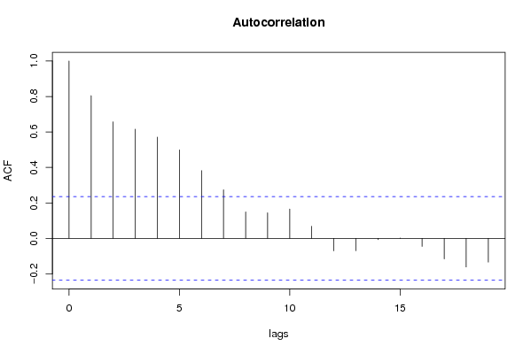
Title produced by software

(Partial) Autocorrelation Function

Date of computation

Sun, 25 Nov 2007 12:07:53 -0700

Cite this page as follows

Statistical Computations at FreeStatistics.org, Office for Research Development and Education, URL https://freestatistics.org/blog/index.php?v=date/2007/Nov/25/t1196017120qnbkxjrt7m7fzxc.htm/, Retrieved Sat, 04 May 2024 14:26:45 +0000

Statistical Computations at FreeStatistics.org, Office for Research Development and Education, URL https://freestatistics.org/blog/index.php?pk=6532, Retrieved Sat, 04 May 2024 14:26:45 +0000

QR Codes:

Paste this QR Code to cite your computation.

Original text written by user:

IsPrivate?

No (this computation is public)

User-defined keywords

Estimated Impact

178

Family? (F = Feedback message, R = changed R code, M = changed R Module, P = changed Parameters, D = changed Data)

-       [(Partial) Autocorrelation Function] [introducing stati...] [2007-11-25 19:07:53] [a04acf73ce4b7e85f8287f21ada159c8] [Current]

Feedback Forum

Post a new message

Dataseries X:

Download CSV

Histogram

Boxplots

Summary of compuational transaction
Raw Input	view raw input (R code)
Raw Output	view raw output of R engine
Computing time	1 seconds
R Server	'Gwilym Jenkins' @ 72.249.127.135

\begin{tabular}{lllllllll}
\hline
Summary of compuational transaction \tabularnewline
Raw Input & view raw input (R code)  \tabularnewline
Raw Output & view raw output of R engine  \tabularnewline
Computing time & 1 seconds \tabularnewline
R Server & 'Gwilym Jenkins' @ 72.249.127.135 \tabularnewline
\hline
\end{tabular}
%Source: https://freestatistics.org/blog/index.php?pk=6532&T=0

[TABLE]
[ROW][C]Summary of compuational transaction[/C][/ROW]
[ROW][C]Raw Input[/C][C]view raw input (R code) [/C][/ROW]
[ROW][C]Raw Output[/C][C]view raw output of R engine [/C][/ROW]
[ROW][C]Computing time[/C][C]1 seconds[/C][/ROW]
[ROW][C]R Server[/C][C]'Gwilym Jenkins' @ 72.249.127.135[/C][/ROW]
[/TABLE]
Source: https://freestatistics.org/blog/index.php?pk=6532&T=0

Globally Unique Identifier (entire table): ba.freestatistics.org/blog/index.php?pk=6532&T=0

As an alternative you can also use a QR Code:

The GUIDs for individual cells are displayed in the table below:

Summary of compuational transaction
Raw Input	view raw input (R code)
Raw Output	view raw output of R engine
Computing time	1 seconds
R Server	'Gwilym Jenkins' @ 72.249.127.135

Autocorrelation Function
Time lag k	ACF(k)	T-STAT	P-value
0	1	8.3066	0
1	0.804544	6.683	0
2	0.657005	5.4575	0
3	0.615794	5.1152	1e-06
4	0.57103	4.7433	5e-06
5	0.498952	4.1446	4.8e-05
6	0.382015	3.1733	0.001126
7	0.273979	2.2758	0.012982
8	0.149578	1.2425	0.109132
9	0.144299	1.1986	0.117384
10	0.165584	1.3754	0.086722
11	0.068424	0.5684	0.285814
12	-0.069965	-0.5812	0.718492
13	-0.069775	-0.5796	0.717963
14	-0.007216	-0.0599	0.523812
15	0.002409	0.02	0.492045
16	-0.04508	-0.3745	0.645396
17	-0.115858	-0.9624	0.830392
18	-0.16123	-1.3393	0.907562

\begin{tabular}{lllllllll}
\hline
Autocorrelation Function \tabularnewline
Time lag k & ACF(k) & T-STAT & P-value \tabularnewline
0 & 1 & 8.3066 & 0 \tabularnewline
1 & 0.804544 & 6.683 & 0 \tabularnewline
2 & 0.657005 & 5.4575 & 0 \tabularnewline
3 & 0.615794 & 5.1152 & 1e-06 \tabularnewline
4 & 0.57103 & 4.7433 & 5e-06 \tabularnewline
5 & 0.498952 & 4.1446 & 4.8e-05 \tabularnewline
6 & 0.382015 & 3.1733 & 0.001126 \tabularnewline
7 & 0.273979 & 2.2758 & 0.012982 \tabularnewline
8 & 0.149578 & 1.2425 & 0.109132 \tabularnewline
9 & 0.144299 & 1.1986 & 0.117384 \tabularnewline
10 & 0.165584 & 1.3754 & 0.086722 \tabularnewline
11 & 0.068424 & 0.5684 & 0.285814 \tabularnewline
12 & -0.069965 & -0.5812 & 0.718492 \tabularnewline
13 & -0.069775 & -0.5796 & 0.717963 \tabularnewline
14 & -0.007216 & -0.0599 & 0.523812 \tabularnewline
15 & 0.002409 & 0.02 & 0.492045 \tabularnewline
16 & -0.04508 & -0.3745 & 0.645396 \tabularnewline
17 & -0.115858 & -0.9624 & 0.830392 \tabularnewline
18 & -0.16123 & -1.3393 & 0.907562 \tabularnewline
\hline
\end{tabular}
%Source: https://freestatistics.org/blog/index.php?pk=6532&T=1

[TABLE]
[ROW][C]Autocorrelation Function[/C][/ROW]
[ROW][C]Time lag k[/C][C]ACF(k)[/C][C]T-STAT[/C][C]P-value[/C][/ROW]
[ROW][C]0[/C][C]1[/C][C]8.3066[/C][C]0[/C][/ROW]
[ROW][C]1[/C][C]0.804544[/C][C]6.683[/C][C]0[/C][/ROW]
[ROW][C]2[/C][C]0.657005[/C][C]5.4575[/C][C]0[/C][/ROW]
[ROW][C]3[/C][C]0.615794[/C][C]5.1152[/C][C]1e-06[/C][/ROW]
[ROW][C]4[/C][C]0.57103[/C][C]4.7433[/C][C]5e-06[/C][/ROW]
[ROW][C]5[/C][C]0.498952[/C][C]4.1446[/C][C]4.8e-05[/C][/ROW]
[ROW][C]6[/C][C]0.382015[/C][C]3.1733[/C][C]0.001126[/C][/ROW]
[ROW][C]7[/C][C]0.273979[/C][C]2.2758[/C][C]0.012982[/C][/ROW]
[ROW][C]8[/C][C]0.149578[/C][C]1.2425[/C][C]0.109132[/C][/ROW]
[ROW][C]9[/C][C]0.144299[/C][C]1.1986[/C][C]0.117384[/C][/ROW]
[ROW][C]10[/C][C]0.165584[/C][C]1.3754[/C][C]0.086722[/C][/ROW]
[ROW][C]11[/C][C]0.068424[/C][C]0.5684[/C][C]0.285814[/C][/ROW]
[ROW][C]12[/C][C]-0.069965[/C][C]-0.5812[/C][C]0.718492[/C][/ROW]
[ROW][C]13[/C][C]-0.069775[/C][C]-0.5796[/C][C]0.717963[/C][/ROW]
[ROW][C]14[/C][C]-0.007216[/C][C]-0.0599[/C][C]0.523812[/C][/ROW]
[ROW][C]15[/C][C]0.002409[/C][C]0.02[/C][C]0.492045[/C][/ROW]
[ROW][C]16[/C][C]-0.04508[/C][C]-0.3745[/C][C]0.645396[/C][/ROW]
[ROW][C]17[/C][C]-0.115858[/C][C]-0.9624[/C][C]0.830392[/C][/ROW]
[ROW][C]18[/C][C]-0.16123[/C][C]-1.3393[/C][C]0.907562[/C][/ROW]
[/TABLE]
Source: https://freestatistics.org/blog/index.php?pk=6532&T=1

Globally Unique Identifier (entire table): ba.freestatistics.org/blog/index.php?pk=6532&T=1

As an alternative you can also use a QR Code:

The GUIDs for individual cells are displayed in the table below:

Autocorrelation Function
Time lag k	ACF(k)	T-STAT	P-value
0	1	8.3066	0
1	0.804544	6.683	0
2	0.657005	5.4575	0
3	0.615794	5.1152	1e-06
4	0.57103	4.7433	5e-06
5	0.498952	4.1446	4.8e-05
6	0.382015	3.1733	0.001126
7	0.273979	2.2758	0.012982
8	0.149578	1.2425	0.109132
9	0.144299	1.1986	0.117384
10	0.165584	1.3754	0.086722
11	0.068424	0.5684	0.285814
12	-0.069965	-0.5812	0.718492
13	-0.069775	-0.5796	0.717963
14	-0.007216	-0.0599	0.523812
15	0.002409	0.02	0.492045
16	-0.04508	-0.3745	0.645396
17	-0.115858	-0.9624	0.830392
18	-0.16123	-1.3393	0.907562

Partial Autocorrelation Function
Time lag k	PACF(k)	T-STAT	P-value
0	0.804544	6.683	0
1	0.02754	0.2288	0.409865
2	0.225865	1.8762	0.032431
3	0.027988	0.2325	0.408426
4	-0.023945	-0.1989	0.578537
5	-0.171354	-1.4234	0.920433
6	-0.104994	-0.8721	0.806922
7	-0.213646	-1.7747	0.959819
8	0.235765	1.9584	0.027113
9	0.118612	0.9853	0.163968
10	-0.149085	-1.2384	0.890116
11	-0.229846	-1.9092	0.969805
12	0.176485	1.466	0.073596
13	0.118543	0.9847	0.164107
14	0.051939	0.4314	0.333747
15	-0.155019	-1.2877	0.898921
16	-0.140177	-1.1644	0.875863
17	-0.088499	-0.7351	0.767624
18	0.087946	0.7305	0.233768

\begin{tabular}{lllllllll}
\hline
Partial Autocorrelation Function \tabularnewline
Time lag k & PACF(k) & T-STAT & P-value \tabularnewline
0 & 0.804544 & 6.683 & 0 \tabularnewline
1 & 0.02754 & 0.2288 & 0.409865 \tabularnewline
2 & 0.225865 & 1.8762 & 0.032431 \tabularnewline
3 & 0.027988 & 0.2325 & 0.408426 \tabularnewline
4 & -0.023945 & -0.1989 & 0.578537 \tabularnewline
5 & -0.171354 & -1.4234 & 0.920433 \tabularnewline
6 & -0.104994 & -0.8721 & 0.806922 \tabularnewline
7 & -0.213646 & -1.7747 & 0.959819 \tabularnewline
8 & 0.235765 & 1.9584 & 0.027113 \tabularnewline
9 & 0.118612 & 0.9853 & 0.163968 \tabularnewline
10 & -0.149085 & -1.2384 & 0.890116 \tabularnewline
11 & -0.229846 & -1.9092 & 0.969805 \tabularnewline
12 & 0.176485 & 1.466 & 0.073596 \tabularnewline
13 & 0.118543 & 0.9847 & 0.164107 \tabularnewline
14 & 0.051939 & 0.4314 & 0.333747 \tabularnewline
15 & -0.155019 & -1.2877 & 0.898921 \tabularnewline
16 & -0.140177 & -1.1644 & 0.875863 \tabularnewline
17 & -0.088499 & -0.7351 & 0.767624 \tabularnewline
18 & 0.087946 & 0.7305 & 0.233768 \tabularnewline
\hline
\end{tabular}
%Source: https://freestatistics.org/blog/index.php?pk=6532&T=2

[TABLE]
[ROW][C]Partial Autocorrelation Function[/C][/ROW]
[ROW][C]Time lag k[/C][C]PACF(k)[/C][C]T-STAT[/C][C]P-value[/C][/ROW]
[ROW][C]0[/C][C]0.804544[/C][C]6.683[/C][C]0[/C][/ROW]
[ROW][C]1[/C][C]0.02754[/C][C]0.2288[/C][C]0.409865[/C][/ROW]
[ROW][C]2[/C][C]0.225865[/C][C]1.8762[/C][C]0.032431[/C][/ROW]
[ROW][C]3[/C][C]0.027988[/C][C]0.2325[/C][C]0.408426[/C][/ROW]
[ROW][C]4[/C][C]-0.023945[/C][C]-0.1989[/C][C]0.578537[/C][/ROW]
[ROW][C]5[/C][C]-0.171354[/C][C]-1.4234[/C][C]0.920433[/C][/ROW]
[ROW][C]6[/C][C]-0.104994[/C][C]-0.8721[/C][C]0.806922[/C][/ROW]
[ROW][C]7[/C][C]-0.213646[/C][C]-1.7747[/C][C]0.959819[/C][/ROW]
[ROW][C]8[/C][C]0.235765[/C][C]1.9584[/C][C]0.027113[/C][/ROW]
[ROW][C]9[/C][C]0.118612[/C][C]0.9853[/C][C]0.163968[/C][/ROW]
[ROW][C]10[/C][C]-0.149085[/C][C]-1.2384[/C][C]0.890116[/C][/ROW]
[ROW][C]11[/C][C]-0.229846[/C][C]-1.9092[/C][C]0.969805[/C][/ROW]
[ROW][C]12[/C][C]0.176485[/C][C]1.466[/C][C]0.073596[/C][/ROW]
[ROW][C]13[/C][C]0.118543[/C][C]0.9847[/C][C]0.164107[/C][/ROW]
[ROW][C]14[/C][C]0.051939[/C][C]0.4314[/C][C]0.333747[/C][/ROW]
[ROW][C]15[/C][C]-0.155019[/C][C]-1.2877[/C][C]0.898921[/C][/ROW]
[ROW][C]16[/C][C]-0.140177[/C][C]-1.1644[/C][C]0.875863[/C][/ROW]
[ROW][C]17[/C][C]-0.088499[/C][C]-0.7351[/C][C]0.767624[/C][/ROW]
[ROW][C]18[/C][C]0.087946[/C][C]0.7305[/C][C]0.233768[/C][/ROW]
[/TABLE]
Source: https://freestatistics.org/blog/index.php?pk=6532&T=2

Globally Unique Identifier (entire table): ba.freestatistics.org/blog/index.php?pk=6532&T=2

As an alternative you can also use a QR Code:

The GUIDs for individual cells are displayed in the table below:

Partial Autocorrelation Function
Time lag k	PACF(k)	T-STAT	P-value
0	0.804544	6.683	0
1	0.02754	0.2288	0.409865
2	0.225865	1.8762	0.032431
3	0.027988	0.2325	0.408426
4	-0.023945	-0.1989	0.578537
5	-0.171354	-1.4234	0.920433
6	-0.104994	-0.8721	0.806922
7	-0.213646	-1.7747	0.959819
8	0.235765	1.9584	0.027113
9	0.118612	0.9853	0.163968
10	-0.149085	-1.2384	0.890116
11	-0.229846	-1.9092	0.969805
12	0.176485	1.466	0.073596
13	0.118543	0.9847	0.164107
14	0.051939	0.4314	0.333747
15	-0.155019	-1.2877	0.898921
16	-0.140177	-1.1644	0.875863
17	-0.088499	-0.7351	0.767624
18	0.087946	0.7305	0.233768

Figure 1

PNG link

Postscript link

PDF link

Figure 2

PNG link

Postscript link

PDF link

Parameters (Session):

par1 = Default ; par2 = 1 ; par3 = 0 ; par4 = 1 ; par5 = 12 ;

Parameters (R input):

par1 = Default ; par2 = 1 ; par3 = 0 ; par4 = 1 ; par5 = 12 ;

R code (references can be found in the software module):

if (par1 == 'Default') {
par1 = 10*log10(length(x))
} else {
par1 <- as.numeric(par1)
}
par2 <- as.numeric(par2)
par3 <- as.numeric(par3)
par4 <- as.numeric(par4)
par5 <- as.numeric(par5)
if (par2 == 0) {
x <- log(x)
} else {
x <- (x ^ par2 - 1) / par2
}
if (par3 > 0) x <- diff(x,lag=1,difference=par3)
if (par4 > 0) x <- diff(x,lag=par5,difference=par4)
bitmap(file='pic1.png')
racf <- acf(x,par1,main='Autocorrelation',xlab='lags',ylab='ACF')
dev.off()
bitmap(file='pic2.png')
rpacf <- pacf(x,par1,main='Partial Autocorrelation',xlab='lags',ylab='PACF')
dev.off()
(myacf <- c(racf$acf))
(mypacf <- c(rpacf$acf))
lengthx <- length(x)
sqrtn <- sqrt(lengthx)
load(file='createtable')
a<-table.start()
a<-table.row.start(a)
a<-table.element(a,'Autocorrelation Function',4,TRUE)
a<-table.row.end(a)
a<-table.row.start(a)
a<-table.element(a,'Time lag k',header=TRUE)
a<-table.element(a,hyperlink('basics.htm','ACF(k)','click here for more information about the Autocorrelation Function'),header=TRUE)
a<-table.element(a,'T-STAT',header=TRUE)
a<-table.element(a,'P-value',header=TRUE)
a<-table.row.end(a)
for (i in 1:par1) {
a<-table.row.start(a)
a<-table.element(a,i-1,header=TRUE)
a<-table.element(a,round(myacf[i],6))
mytstat <- myacf[i]*sqrtn
a<-table.element(a,round(mytstat,4))
a<-table.element(a,round(1-pt(mytstat,lengthx),6))
a<-table.row.end(a)
}
a<-table.end(a)
table.save(a,file='mytable.tab')
a<-table.start()
a<-table.row.start(a)
a<-table.element(a,'Partial Autocorrelation Function',4,TRUE)
a<-table.row.end(a)
a<-table.row.start(a)
a<-table.element(a,'Time lag k',header=TRUE)
a<-table.element(a,hyperlink('basics.htm','PACF(k)','click here for more information about the Partial Autocorrelation Function'),header=TRUE)
a<-table.element(a,'T-STAT',header=TRUE)
a<-table.element(a,'P-value',header=TRUE)
a<-table.row.end(a)
for (i in 1:par1) {
a<-table.row.start(a)
a<-table.element(a,i-1,header=TRUE)
a<-table.element(a,round(mypacf[i],6))
mytstat <- mypacf[i]*sqrtn
a<-table.element(a,round(mytstat,4))
a<-table.element(a,round(1-pt(mytstat,lengthx),6))
a<-table.row.end(a)
}
a<-table.end(a)
table.save(a,file='mytable1.tab')

Free Statistics

Description of Statistical Computation

Tree of Dependent Computations

Dataset

Tables (Output of Computation)

Figures (Output of Computation)

Input Parameters & R Code