Repository of Reproducible Computations

Free Statistics

of Irreproducible Research!

Author's title

Author

*Unverified author*

R Software Module

rwasp_autocorrelation.wasp

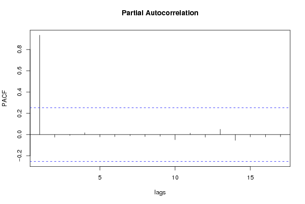
Title produced by software

(Partial) Autocorrelation Function

Date of computation

Sat, 24 Nov 2007 07:11:14 -0700

Cite this page as follows

Statistical Computations at FreeStatistics.org, Office for Research Development and Education, URL https://freestatistics.org/blog/index.php?v=date/2007/Nov/24/t1195913014ygv2vqe69uirqdz.htm/, Retrieved Fri, 03 May 2024 05:57:06 +0000

Statistical Computations at FreeStatistics.org, Office for Research Development and Education, URL https://freestatistics.org/blog/index.php?pk=6305, Retrieved Fri, 03 May 2024 05:57:06 +0000

QR Codes:

Paste this QR Code to cite your computation.

Original text written by user:

IsPrivate?

No (this computation is public)

User-defined keywords

G19Q2

Estimated Impact

185

Family? (F = Feedback message, R = changed R code, M = changed R Module, P = changed Parameters, D = changed Data)

-       [(Partial) Autocorrelation Function] [Partial Autocorre...] [2007-11-24 14:11:14] [6b5c00822e2ce0f7cf73539c28d95782] [Current]

Feedback Forum

Post a new message

Dataseries X:

Download CSV

Histogram

Boxplots

Summary of compuational transaction
Raw Input	view raw input (R code)
Raw Output	view raw output of R engine
Computing time	1 seconds
R Server	'Gwilym Jenkins' @ 72.249.127.135

\begin{tabular}{lllllllll}
\hline
Summary of compuational transaction \tabularnewline
Raw Input & view raw input (R code)  \tabularnewline
Raw Output & view raw output of R engine  \tabularnewline
Computing time & 1 seconds \tabularnewline
R Server & 'Gwilym Jenkins' @ 72.249.127.135 \tabularnewline
\hline
\end{tabular}
%Source: https://freestatistics.org/blog/index.php?pk=6305&T=0

[TABLE]
[ROW][C]Summary of compuational transaction[/C][/ROW]
[ROW][C]Raw Input[/C][C]view raw input (R code) [/C][/ROW]
[ROW][C]Raw Output[/C][C]view raw output of R engine [/C][/ROW]
[ROW][C]Computing time[/C][C]1 seconds[/C][/ROW]
[ROW][C]R Server[/C][C]'Gwilym Jenkins' @ 72.249.127.135[/C][/ROW]
[/TABLE]
Source: https://freestatistics.org/blog/index.php?pk=6305&T=0

Globally Unique Identifier (entire table): ba.freestatistics.org/blog/index.php?pk=6305&T=0

As an alternative you can also use a QR Code:

The GUIDs for individual cells are displayed in the table below:

Summary of compuational transaction
Raw Input	view raw input (R code)
Raw Output	view raw output of R engine
Computing time	1 seconds
R Server	'Gwilym Jenkins' @ 72.249.127.135

Autocorrelation Function
Time lag k	ACF(k)	T-STAT	P-value
0	1	7.746	0
1	0.934735	7.2404	0
2	0.870588	6.7435	0
3	0.809725	6.2721	0
4	0.7553	5.8505	0
5	0.7019	5.4369	1e-06
6	0.649667	5.0323	2e-06
7	0.599657	4.6449	1e-05
8	0.550947	4.2676	3.6e-05
9	0.503972	3.9037	0.000121
10	0.45455	3.5209	0.000414
11	0.41086	3.1825	0.001157
12	0.367796	2.8489	0.003001
13	0.334942	2.5944	0.005945
14	0.298018	2.3084	0.012219
15	0.261525	2.0258	0.023621
16	0.225253	1.7448	0.04307

\begin{tabular}{lllllllll}
\hline
Autocorrelation Function \tabularnewline
Time lag k & ACF(k) & T-STAT & P-value \tabularnewline
0 & 1 & 7.746 & 0 \tabularnewline
1 & 0.934735 & 7.2404 & 0 \tabularnewline
2 & 0.870588 & 6.7435 & 0 \tabularnewline
3 & 0.809725 & 6.2721 & 0 \tabularnewline
4 & 0.7553 & 5.8505 & 0 \tabularnewline
5 & 0.7019 & 5.4369 & 1e-06 \tabularnewline
6 & 0.649667 & 5.0323 & 2e-06 \tabularnewline
7 & 0.599657 & 4.6449 & 1e-05 \tabularnewline
8 & 0.550947 & 4.2676 & 3.6e-05 \tabularnewline
9 & 0.503972 & 3.9037 & 0.000121 \tabularnewline
10 & 0.45455 & 3.5209 & 0.000414 \tabularnewline
11 & 0.41086 & 3.1825 & 0.001157 \tabularnewline
12 & 0.367796 & 2.8489 & 0.003001 \tabularnewline
13 & 0.334942 & 2.5944 & 0.005945 \tabularnewline
14 & 0.298018 & 2.3084 & 0.012219 \tabularnewline
15 & 0.261525 & 2.0258 & 0.023621 \tabularnewline
16 & 0.225253 & 1.7448 & 0.04307 \tabularnewline
\hline
\end{tabular}
%Source: https://freestatistics.org/blog/index.php?pk=6305&T=1

[TABLE]
[ROW][C]Autocorrelation Function[/C][/ROW]
[ROW][C]Time lag k[/C][C]ACF(k)[/C][C]T-STAT[/C][C]P-value[/C][/ROW]
[ROW][C]0[/C][C]1[/C][C]7.746[/C][C]0[/C][/ROW]
[ROW][C]1[/C][C]0.934735[/C][C]7.2404[/C][C]0[/C][/ROW]
[ROW][C]2[/C][C]0.870588[/C][C]6.7435[/C][C]0[/C][/ROW]
[ROW][C]3[/C][C]0.809725[/C][C]6.2721[/C][C]0[/C][/ROW]
[ROW][C]4[/C][C]0.7553[/C][C]5.8505[/C][C]0[/C][/ROW]
[ROW][C]5[/C][C]0.7019[/C][C]5.4369[/C][C]1e-06[/C][/ROW]
[ROW][C]6[/C][C]0.649667[/C][C]5.0323[/C][C]2e-06[/C][/ROW]
[ROW][C]7[/C][C]0.599657[/C][C]4.6449[/C][C]1e-05[/C][/ROW]
[ROW][C]8[/C][C]0.550947[/C][C]4.2676[/C][C]3.6e-05[/C][/ROW]
[ROW][C]9[/C][C]0.503972[/C][C]3.9037[/C][C]0.000121[/C][/ROW]
[ROW][C]10[/C][C]0.45455[/C][C]3.5209[/C][C]0.000414[/C][/ROW]
[ROW][C]11[/C][C]0.41086[/C][C]3.1825[/C][C]0.001157[/C][/ROW]
[ROW][C]12[/C][C]0.367796[/C][C]2.8489[/C][C]0.003001[/C][/ROW]
[ROW][C]13[/C][C]0.334942[/C][C]2.5944[/C][C]0.005945[/C][/ROW]
[ROW][C]14[/C][C]0.298018[/C][C]2.3084[/C][C]0.012219[/C][/ROW]
[ROW][C]15[/C][C]0.261525[/C][C]2.0258[/C][C]0.023621[/C][/ROW]
[ROW][C]16[/C][C]0.225253[/C][C]1.7448[/C][C]0.04307[/C][/ROW]
[/TABLE]
Source: https://freestatistics.org/blog/index.php?pk=6305&T=1

Globally Unique Identifier (entire table): ba.freestatistics.org/blog/index.php?pk=6305&T=1

As an alternative you can also use a QR Code:

The GUIDs for individual cells are displayed in the table below:

Autocorrelation Function
Time lag k	ACF(k)	T-STAT	P-value
0	1	7.746	0
1	0.934735	7.2404	0
2	0.870588	6.7435	0
3	0.809725	6.2721	0
4	0.7553	5.8505	0
5	0.7019	5.4369	1e-06
6	0.649667	5.0323	2e-06
7	0.599657	4.6449	1e-05
8	0.550947	4.2676	3.6e-05
9	0.503972	3.9037	0.000121
10	0.45455	3.5209	0.000414
11	0.41086	3.1825	0.001157
12	0.367796	2.8489	0.003001
13	0.334942	2.5944	0.005945
14	0.298018	2.3084	0.012219
15	0.261525	2.0258	0.023621
16	0.225253	1.7448	0.04307

Partial Autocorrelation Function
Time lag k	PACF(k)	T-STAT	P-value
0	0.934735	7.2404	0
1	-0.024873	-0.1927	0.576064
2	-0.008203	-0.0635	0.525227
3	0.017766	0.1376	0.445503
4	-0.021721	-0.1682	0.566523
5	-0.019817	-0.1535	0.560742
6	-0.011267	-0.0873	0.534627
7	-0.019665	-0.1523	0.560279
8	-0.015906	-0.1232	0.548822
9	-0.048472	-0.3755	0.64568
10	0.013366	0.1035	0.458942
11	-0.02511	-0.1945	0.576779
12	0.050192	0.3888	0.349405
13	-0.053959	-0.418	0.661268
14	-0.021589	-0.1672	0.566124
15	-0.022172	-0.1717	0.567891
16	-0.020479	-0.1586	0.562753

\begin{tabular}{lllllllll}
\hline
Partial Autocorrelation Function \tabularnewline
Time lag k & PACF(k) & T-STAT & P-value \tabularnewline
0 & 0.934735 & 7.2404 & 0 \tabularnewline
1 & -0.024873 & -0.1927 & 0.576064 \tabularnewline
2 & -0.008203 & -0.0635 & 0.525227 \tabularnewline
3 & 0.017766 & 0.1376 & 0.445503 \tabularnewline
4 & -0.021721 & -0.1682 & 0.566523 \tabularnewline
5 & -0.019817 & -0.1535 & 0.560742 \tabularnewline
6 & -0.011267 & -0.0873 & 0.534627 \tabularnewline
7 & -0.019665 & -0.1523 & 0.560279 \tabularnewline
8 & -0.015906 & -0.1232 & 0.548822 \tabularnewline
9 & -0.048472 & -0.3755 & 0.64568 \tabularnewline
10 & 0.013366 & 0.1035 & 0.458942 \tabularnewline
11 & -0.02511 & -0.1945 & 0.576779 \tabularnewline
12 & 0.050192 & 0.3888 & 0.349405 \tabularnewline
13 & -0.053959 & -0.418 & 0.661268 \tabularnewline
14 & -0.021589 & -0.1672 & 0.566124 \tabularnewline
15 & -0.022172 & -0.1717 & 0.567891 \tabularnewline
16 & -0.020479 & -0.1586 & 0.562753 \tabularnewline
\hline
\end{tabular}
%Source: https://freestatistics.org/blog/index.php?pk=6305&T=2

[TABLE]
[ROW][C]Partial Autocorrelation Function[/C][/ROW]
[ROW][C]Time lag k[/C][C]PACF(k)[/C][C]T-STAT[/C][C]P-value[/C][/ROW]
[ROW][C]0[/C][C]0.934735[/C][C]7.2404[/C][C]0[/C][/ROW]
[ROW][C]1[/C][C]-0.024873[/C][C]-0.1927[/C][C]0.576064[/C][/ROW]
[ROW][C]2[/C][C]-0.008203[/C][C]-0.0635[/C][C]0.525227[/C][/ROW]
[ROW][C]3[/C][C]0.017766[/C][C]0.1376[/C][C]0.445503[/C][/ROW]
[ROW][C]4[/C][C]-0.021721[/C][C]-0.1682[/C][C]0.566523[/C][/ROW]
[ROW][C]5[/C][C]-0.019817[/C][C]-0.1535[/C][C]0.560742[/C][/ROW]
[ROW][C]6[/C][C]-0.011267[/C][C]-0.0873[/C][C]0.534627[/C][/ROW]
[ROW][C]7[/C][C]-0.019665[/C][C]-0.1523[/C][C]0.560279[/C][/ROW]
[ROW][C]8[/C][C]-0.015906[/C][C]-0.1232[/C][C]0.548822[/C][/ROW]
[ROW][C]9[/C][C]-0.048472[/C][C]-0.3755[/C][C]0.64568[/C][/ROW]
[ROW][C]10[/C][C]0.013366[/C][C]0.1035[/C][C]0.458942[/C][/ROW]
[ROW][C]11[/C][C]-0.02511[/C][C]-0.1945[/C][C]0.576779[/C][/ROW]
[ROW][C]12[/C][C]0.050192[/C][C]0.3888[/C][C]0.349405[/C][/ROW]
[ROW][C]13[/C][C]-0.053959[/C][C]-0.418[/C][C]0.661268[/C][/ROW]
[ROW][C]14[/C][C]-0.021589[/C][C]-0.1672[/C][C]0.566124[/C][/ROW]
[ROW][C]15[/C][C]-0.022172[/C][C]-0.1717[/C][C]0.567891[/C][/ROW]
[ROW][C]16[/C][C]-0.020479[/C][C]-0.1586[/C][C]0.562753[/C][/ROW]
[/TABLE]
Source: https://freestatistics.org/blog/index.php?pk=6305&T=2

Globally Unique Identifier (entire table): ba.freestatistics.org/blog/index.php?pk=6305&T=2

As an alternative you can also use a QR Code:

The GUIDs for individual cells are displayed in the table below:

Partial Autocorrelation Function
Time lag k	PACF(k)	T-STAT	P-value
0	0.934735	7.2404	0
1	-0.024873	-0.1927	0.576064
2	-0.008203	-0.0635	0.525227
3	0.017766	0.1376	0.445503
4	-0.021721	-0.1682	0.566523
5	-0.019817	-0.1535	0.560742
6	-0.011267	-0.0873	0.534627
7	-0.019665	-0.1523	0.560279
8	-0.015906	-0.1232	0.548822
9	-0.048472	-0.3755	0.64568
10	0.013366	0.1035	0.458942
11	-0.02511	-0.1945	0.576779
12	0.050192	0.3888	0.349405
13	-0.053959	-0.418	0.661268
14	-0.021589	-0.1672	0.566124
15	-0.022172	-0.1717	0.567891
16	-0.020479	-0.1586	0.562753

Figure 1

PNG link

Postscript link

PDF link

Figure 2

PNG link

Postscript link

PDF link

Parameters (Session):

par1 = Default ; par2 = 1 ; par3 = 0 ; par4 = 0 ; par5 = 12 ;

Parameters (R input):

par1 = Default ; par2 = 1 ; par3 = 0 ; par4 = 0 ; par5 = 12 ;

R code (references can be found in the software module):

if (par1 == 'Default') {
par1 = 10*log10(length(x))
} else {
par1 <- as.numeric(par1)
}
par2 <- as.numeric(par2)
par3 <- as.numeric(par3)
par4 <- as.numeric(par4)
par5 <- as.numeric(par5)
if (par2 == 0) {
x <- log(x)
} else {
x <- (x ^ par2 - 1) / par2
}
if (par3 > 0) x <- diff(x,lag=1,difference=par3)
if (par4 > 0) x <- diff(x,lag=par5,difference=par4)
bitmap(file='pic1.png')
racf <- acf(x,par1,main='Autocorrelation',xlab='lags',ylab='ACF')
dev.off()
bitmap(file='pic2.png')
rpacf <- pacf(x,par1,main='Partial Autocorrelation',xlab='lags',ylab='PACF')
dev.off()
(myacf <- c(racf$acf))
(mypacf <- c(rpacf$acf))
lengthx <- length(x)
sqrtn <- sqrt(lengthx)
load(file='createtable')
a<-table.start()
a<-table.row.start(a)
a<-table.element(a,'Autocorrelation Function',4,TRUE)
a<-table.row.end(a)
a<-table.row.start(a)
a<-table.element(a,'Time lag k',header=TRUE)
a<-table.element(a,hyperlink('basics.htm','ACF(k)','click here for more information about the Autocorrelation Function'),header=TRUE)
a<-table.element(a,'T-STAT',header=TRUE)
a<-table.element(a,'P-value',header=TRUE)
a<-table.row.end(a)
for (i in 1:par1) {
a<-table.row.start(a)
a<-table.element(a,i-1,header=TRUE)
a<-table.element(a,round(myacf[i],6))
mytstat <- myacf[i]*sqrtn
a<-table.element(a,round(mytstat,4))
a<-table.element(a,round(1-pt(mytstat,lengthx),6))
a<-table.row.end(a)
}
a<-table.end(a)
table.save(a,file='mytable.tab')
a<-table.start()
a<-table.row.start(a)
a<-table.element(a,'Partial Autocorrelation Function',4,TRUE)
a<-table.row.end(a)
a<-table.row.start(a)
a<-table.element(a,'Time lag k',header=TRUE)
a<-table.element(a,hyperlink('basics.htm','PACF(k)','click here for more information about the Partial Autocorrelation Function'),header=TRUE)
a<-table.element(a,'T-STAT',header=TRUE)
a<-table.element(a,'P-value',header=TRUE)
a<-table.row.end(a)
for (i in 1:par1) {
a<-table.row.start(a)
a<-table.element(a,i-1,header=TRUE)
a<-table.element(a,round(mypacf[i],6))
mytstat <- mypacf[i]*sqrtn
a<-table.element(a,round(mytstat,4))
a<-table.element(a,round(1-pt(mytstat,lengthx),6))
a<-table.row.end(a)
}
a<-table.end(a)
table.save(a,file='mytable1.tab')

Free Statistics

Description of Statistical Computation

Tree of Dependent Computations

Dataset

Tables (Output of Computation)

Figures (Output of Computation)

Input Parameters & R Code