Free Statistics
of Irreproducible Research!
Description of Statistical Computation | |||||||||||||||||||||||||||||||||||||
|---|---|---|---|---|---|---|---|---|---|---|---|---|---|---|---|---|---|---|---|---|---|---|---|---|---|---|---|---|---|---|---|---|---|---|---|---|---|
| Author's title | |||||||||||||||||||||||||||||||||||||
| Author | *Unverified author* | ||||||||||||||||||||||||||||||||||||
| R Software Module | rwasp_boxcoxnorm.wasp | ||||||||||||||||||||||||||||||||||||
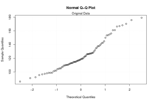
| Title produced by software | Box-Cox Normality Plot | ||||||||||||||||||||||||||||||||||||
| Date of computation | Sat, 24 Nov 2007 06:20:50 -0700 | ||||||||||||||||||||||||||||||||||||
| Cite this page as follows | Statistical Computations at FreeStatistics.org, Office for Research Development and Education, URL https://freestatistics.org/blog/index.php?v=date/2007/Nov/24/t1195909951f7j059nu5bxk75t.htm/, Retrieved Fri, 03 May 2024 12:12:32 +0000 | ||||||||||||||||||||||||||||||||||||
| Statistical Computations at FreeStatistics.org, Office for Research Development and Education, URL https://freestatistics.org/blog/index.php?pk=6286, Retrieved Fri, 03 May 2024 12:12:32 +0000 | |||||||||||||||||||||||||||||||||||||
| QR Codes: | |||||||||||||||||||||||||||||||||||||
|
| |||||||||||||||||||||||||||||||||||||
| Original text written by user: | |||||||||||||||||||||||||||||||||||||
| IsPrivate? | No (this computation is public) | ||||||||||||||||||||||||||||||||||||
| User-defined keywords | WS7BCM | ||||||||||||||||||||||||||||||||||||
| Estimated Impact | 238 | ||||||||||||||||||||||||||||||||||||
Tree of Dependent Computations | |||||||||||||||||||||||||||||||||||||
| Family? (F = Feedback message, R = changed R code, M = changed R Module, P = changed Parameters, D = changed Data) | |||||||||||||||||||||||||||||||||||||
| - [Box-Cox Normality Plot] [WS7 - BC - Medical] [2007-11-24 13:20:50] [e51d7ab0e549b3dc96ac85a81d9bd259] [Current] | |||||||||||||||||||||||||||||||||||||
| Feedback Forum | |||||||||||||||||||||||||||||||||||||
Post a new message | |||||||||||||||||||||||||||||||||||||
Dataset | |||||||||||||||||||||||||||||||||||||
| Dataseries X: | |||||||||||||||||||||||||||||||||||||
96,5 97,3 122,0 91,0 107,9 114,6 98,0 95,5 98,7 115,9 110,4 109,5 92,3 102,1 112,8 110,2 98,9 119,0 104,3 98,8 109,4 170,3 118,0 116,9 111,7 116,8 116,1 114,8 110,8 122,8 104,7 86,0 127,2 126,1 114,6 127,8 105,2 113,1 161,0 126,9 117,7 144,9 119,4 107,1 142,8 126,2 126,9 179,2 105,3 114,8 125,4 113,2 134,4 150,0 100,9 101,8 137,7 138,7 135,4 153,8 119,5 123,3 166,4 137,5 142,2 167,0 112,3 120,6 154,9 153,4 156,2 175,8 131,7 130,1 161,1 128,2 140,3 168,2 110,2 126,2 | |||||||||||||||||||||||||||||||||||||
Tables (Output of Computation) | |||||||||||||||||||||||||||||||||||||
| |||||||||||||||||||||||||||||||||||||
Figures (Output of Computation) | |||||||||||||||||||||||||||||||||||||
Input Parameters & R Code | |||||||||||||||||||||||||||||||||||||
| Parameters (Session): | |||||||||||||||||||||||||||||||||||||
| Parameters (R input): | |||||||||||||||||||||||||||||||||||||
| R code (references can be found in the software module): | |||||||||||||||||||||||||||||||||||||
n <- length(x) | |||||||||||||||||||||||||||||||||||||