Repository of Reproducible Computations

Free Statistics

of Irreproducible Research!

Author's title

Author

*Unverified author*

R Software Module

rwasp_autocorrelation.wasp

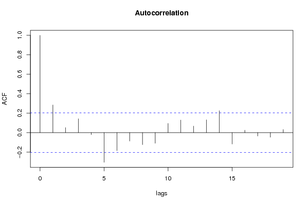
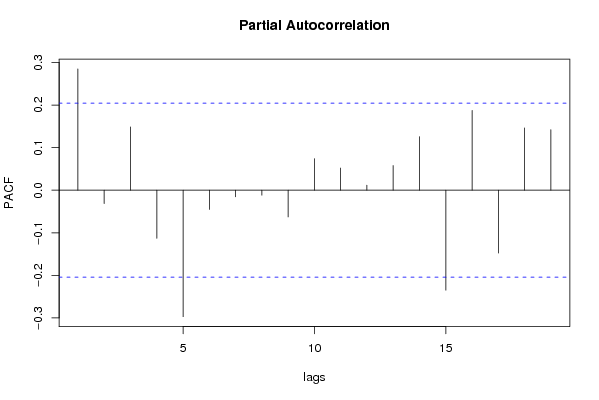
Title produced by software

(Partial) Autocorrelation Function

Date of computation

Fri, 23 Nov 2007 06:03:43 -0700

Cite this page as follows

Statistical Computations at FreeStatistics.org, Office for Research Development and Education, URL https://freestatistics.org/blog/index.php?v=date/2007/Nov/23/t1195822521k0bcaahcymp9tcw.htm/, Retrieved Mon, 29 Apr 2024 00:05:08 +0000

Statistical Computations at FreeStatistics.org, Office for Research Development and Education, URL https://freestatistics.org/blog/index.php?pk=6157, Retrieved Mon, 29 Apr 2024 00:05:08 +0000

QR Codes:

Paste this QR Code to cite your computation.

Original text written by user:

IsPrivate?

No (this computation is public)

User-defined keywords

Estimated Impact

233

Family? (F = Feedback message, R = changed R code, M = changed R Module, P = changed Parameters, D = changed Data)

-       [(Partial) Autocorrelation Function] [] [2007-11-23 13:03:43] [22d719c250b0837edaa2d173fd414084] [Current]

Feedback Forum

Post a new message

Dataseries X:

Download CSV

Histogram

Boxplots

Summary of compuational transaction
Raw Input	view raw input (R code)
Raw Output	view raw output of R engine
Computing time	1 seconds
R Server	'Gwilym Jenkins' @ 72.249.127.135

\begin{tabular}{lllllllll}
\hline
Summary of compuational transaction \tabularnewline
Raw Input & view raw input (R code)  \tabularnewline
Raw Output & view raw output of R engine  \tabularnewline
Computing time & 1 seconds \tabularnewline
R Server & 'Gwilym Jenkins' @ 72.249.127.135 \tabularnewline
\hline
\end{tabular}
%Source: https://freestatistics.org/blog/index.php?pk=6157&T=0

[TABLE]
[ROW][C]Summary of compuational transaction[/C][/ROW]
[ROW][C]Raw Input[/C][C]view raw input (R code) [/C][/ROW]
[ROW][C]Raw Output[/C][C]view raw output of R engine [/C][/ROW]
[ROW][C]Computing time[/C][C]1 seconds[/C][/ROW]
[ROW][C]R Server[/C][C]'Gwilym Jenkins' @ 72.249.127.135[/C][/ROW]
[/TABLE]
Source: https://freestatistics.org/blog/index.php?pk=6157&T=0

Globally Unique Identifier (entire table): ba.freestatistics.org/blog/index.php?pk=6157&T=0

As an alternative you can also use a QR Code:

The GUIDs for individual cells are displayed in the table below:

Summary of compuational transaction
Raw Input	view raw input (R code)
Raw Output	view raw output of R engine
Computing time	1 seconds
R Server	'Gwilym Jenkins' @ 72.249.127.135

Autocorrelation Function
Time lag k	ACF(k)	T-STAT	P-value
0	1	9.5917	0
1	0.284676	2.7305	0.003789
2	0.052198	0.5007	0.308901
3	0.142631	1.3681	0.087311
4	-0.020495	-0.1966	0.577705
5	-0.304248	-2.9182	0.997788
6	-0.184722	-1.7718	0.96013
7	-0.086861	-0.8331	0.796539
8	-0.12315	-1.1812	0.879719
9	-0.108707	-1.0427	0.850085
10	0.09502	0.9114	0.182234
11	0.130213	1.249	0.107425
12	0.067257	0.6451	0.260233
13	0.132045	1.2665	0.104261
14	0.226148	2.1691	0.016325
15	-0.116631	-1.1187	0.866906
16	0.025221	0.2419	0.404693
17	-0.034873	-0.3345	0.630614
18	-0.047375	-0.4544	0.674694

\begin{tabular}{lllllllll}
\hline
Autocorrelation Function \tabularnewline
Time lag k & ACF(k) & T-STAT & P-value \tabularnewline
0 & 1 & 9.5917 & 0 \tabularnewline
1 & 0.284676 & 2.7305 & 0.003789 \tabularnewline
2 & 0.052198 & 0.5007 & 0.308901 \tabularnewline
3 & 0.142631 & 1.3681 & 0.087311 \tabularnewline
4 & -0.020495 & -0.1966 & 0.577705 \tabularnewline
5 & -0.304248 & -2.9182 & 0.997788 \tabularnewline
6 & -0.184722 & -1.7718 & 0.96013 \tabularnewline
7 & -0.086861 & -0.8331 & 0.796539 \tabularnewline
8 & -0.12315 & -1.1812 & 0.879719 \tabularnewline
9 & -0.108707 & -1.0427 & 0.850085 \tabularnewline
10 & 0.09502 & 0.9114 & 0.182234 \tabularnewline
11 & 0.130213 & 1.249 & 0.107425 \tabularnewline
12 & 0.067257 & 0.6451 & 0.260233 \tabularnewline
13 & 0.132045 & 1.2665 & 0.104261 \tabularnewline
14 & 0.226148 & 2.1691 & 0.016325 \tabularnewline
15 & -0.116631 & -1.1187 & 0.866906 \tabularnewline
16 & 0.025221 & 0.2419 & 0.404693 \tabularnewline
17 & -0.034873 & -0.3345 & 0.630614 \tabularnewline
18 & -0.047375 & -0.4544 & 0.674694 \tabularnewline
\hline
\end{tabular}
%Source: https://freestatistics.org/blog/index.php?pk=6157&T=1

[TABLE]
[ROW][C]Autocorrelation Function[/C][/ROW]
[ROW][C]Time lag k[/C][C]ACF(k)[/C][C]T-STAT[/C][C]P-value[/C][/ROW]
[ROW][C]0[/C][C]1[/C][C]9.5917[/C][C]0[/C][/ROW]
[ROW][C]1[/C][C]0.284676[/C][C]2.7305[/C][C]0.003789[/C][/ROW]
[ROW][C]2[/C][C]0.052198[/C][C]0.5007[/C][C]0.308901[/C][/ROW]
[ROW][C]3[/C][C]0.142631[/C][C]1.3681[/C][C]0.087311[/C][/ROW]
[ROW][C]4[/C][C]-0.020495[/C][C]-0.1966[/C][C]0.577705[/C][/ROW]
[ROW][C]5[/C][C]-0.304248[/C][C]-2.9182[/C][C]0.997788[/C][/ROW]
[ROW][C]6[/C][C]-0.184722[/C][C]-1.7718[/C][C]0.96013[/C][/ROW]
[ROW][C]7[/C][C]-0.086861[/C][C]-0.8331[/C][C]0.796539[/C][/ROW]
[ROW][C]8[/C][C]-0.12315[/C][C]-1.1812[/C][C]0.879719[/C][/ROW]
[ROW][C]9[/C][C]-0.108707[/C][C]-1.0427[/C][C]0.850085[/C][/ROW]
[ROW][C]10[/C][C]0.09502[/C][C]0.9114[/C][C]0.182234[/C][/ROW]
[ROW][C]11[/C][C]0.130213[/C][C]1.249[/C][C]0.107425[/C][/ROW]
[ROW][C]12[/C][C]0.067257[/C][C]0.6451[/C][C]0.260233[/C][/ROW]
[ROW][C]13[/C][C]0.132045[/C][C]1.2665[/C][C]0.104261[/C][/ROW]
[ROW][C]14[/C][C]0.226148[/C][C]2.1691[/C][C]0.016325[/C][/ROW]
[ROW][C]15[/C][C]-0.116631[/C][C]-1.1187[/C][C]0.866906[/C][/ROW]
[ROW][C]16[/C][C]0.025221[/C][C]0.2419[/C][C]0.404693[/C][/ROW]
[ROW][C]17[/C][C]-0.034873[/C][C]-0.3345[/C][C]0.630614[/C][/ROW]
[ROW][C]18[/C][C]-0.047375[/C][C]-0.4544[/C][C]0.674694[/C][/ROW]
[/TABLE]
Source: https://freestatistics.org/blog/index.php?pk=6157&T=1

Globally Unique Identifier (entire table): ba.freestatistics.org/blog/index.php?pk=6157&T=1

As an alternative you can also use a QR Code:

The GUIDs for individual cells are displayed in the table below:

Autocorrelation Function
Time lag k	ACF(k)	T-STAT	P-value
0	1	9.5917	0
1	0.284676	2.7305	0.003789
2	0.052198	0.5007	0.308901
3	0.142631	1.3681	0.087311
4	-0.020495	-0.1966	0.577705
5	-0.304248	-2.9182	0.997788
6	-0.184722	-1.7718	0.96013
7	-0.086861	-0.8331	0.796539
8	-0.12315	-1.1812	0.879719
9	-0.108707	-1.0427	0.850085
10	0.09502	0.9114	0.182234
11	0.130213	1.249	0.107425
12	0.067257	0.6451	0.260233
13	0.132045	1.2665	0.104261
14	0.226148	2.1691	0.016325
15	-0.116631	-1.1187	0.866906
16	0.025221	0.2419	0.404693
17	-0.034873	-0.3345	0.630614
18	-0.047375	-0.4544	0.674694

Partial Autocorrelation Function
Time lag k	PACF(k)	T-STAT	P-value
0	0.284676	2.7305	0.003789
1	-0.031386	-0.301	0.617969
2	0.148401	1.4234	0.079
3	-0.112905	-1.083	0.85917
4	-0.296997	-2.8487	0.997292
5	-0.045235	-0.4339	0.667303
6	-0.015506	-0.1487	0.558952
7	-0.011905	-0.1142	0.545331
8	-0.062752	-0.6019	0.725639
9	0.073821	0.7081	0.240348
10	0.052015	0.4989	0.309516
11	0.011782	0.113	0.455135
12	0.057734	0.5538	0.290541
13	0.125496	1.2037	0.115893
14	-0.234921	-2.2533	0.986691
15	0.187344	1.7969	0.037813
16	-0.147707	-1.4168	0.920034
17	0.146041	1.4008	0.082323
18	0.142076	1.3627	0.088144

\begin{tabular}{lllllllll}
\hline
Partial Autocorrelation Function \tabularnewline
Time lag k & PACF(k) & T-STAT & P-value \tabularnewline
0 & 0.284676 & 2.7305 & 0.003789 \tabularnewline
1 & -0.031386 & -0.301 & 0.617969 \tabularnewline
2 & 0.148401 & 1.4234 & 0.079 \tabularnewline
3 & -0.112905 & -1.083 & 0.85917 \tabularnewline
4 & -0.296997 & -2.8487 & 0.997292 \tabularnewline
5 & -0.045235 & -0.4339 & 0.667303 \tabularnewline
6 & -0.015506 & -0.1487 & 0.558952 \tabularnewline
7 & -0.011905 & -0.1142 & 0.545331 \tabularnewline
8 & -0.062752 & -0.6019 & 0.725639 \tabularnewline
9 & 0.073821 & 0.7081 & 0.240348 \tabularnewline
10 & 0.052015 & 0.4989 & 0.309516 \tabularnewline
11 & 0.011782 & 0.113 & 0.455135 \tabularnewline
12 & 0.057734 & 0.5538 & 0.290541 \tabularnewline
13 & 0.125496 & 1.2037 & 0.115893 \tabularnewline
14 & -0.234921 & -2.2533 & 0.986691 \tabularnewline
15 & 0.187344 & 1.7969 & 0.037813 \tabularnewline
16 & -0.147707 & -1.4168 & 0.920034 \tabularnewline
17 & 0.146041 & 1.4008 & 0.082323 \tabularnewline
18 & 0.142076 & 1.3627 & 0.088144 \tabularnewline
\hline
\end{tabular}
%Source: https://freestatistics.org/blog/index.php?pk=6157&T=2

[TABLE]
[ROW][C]Partial Autocorrelation Function[/C][/ROW]
[ROW][C]Time lag k[/C][C]PACF(k)[/C][C]T-STAT[/C][C]P-value[/C][/ROW]
[ROW][C]0[/C][C]0.284676[/C][C]2.7305[/C][C]0.003789[/C][/ROW]
[ROW][C]1[/C][C]-0.031386[/C][C]-0.301[/C][C]0.617969[/C][/ROW]
[ROW][C]2[/C][C]0.148401[/C][C]1.4234[/C][C]0.079[/C][/ROW]
[ROW][C]3[/C][C]-0.112905[/C][C]-1.083[/C][C]0.85917[/C][/ROW]
[ROW][C]4[/C][C]-0.296997[/C][C]-2.8487[/C][C]0.997292[/C][/ROW]
[ROW][C]5[/C][C]-0.045235[/C][C]-0.4339[/C][C]0.667303[/C][/ROW]
[ROW][C]6[/C][C]-0.015506[/C][C]-0.1487[/C][C]0.558952[/C][/ROW]
[ROW][C]7[/C][C]-0.011905[/C][C]-0.1142[/C][C]0.545331[/C][/ROW]
[ROW][C]8[/C][C]-0.062752[/C][C]-0.6019[/C][C]0.725639[/C][/ROW]
[ROW][C]9[/C][C]0.073821[/C][C]0.7081[/C][C]0.240348[/C][/ROW]
[ROW][C]10[/C][C]0.052015[/C][C]0.4989[/C][C]0.309516[/C][/ROW]
[ROW][C]11[/C][C]0.011782[/C][C]0.113[/C][C]0.455135[/C][/ROW]
[ROW][C]12[/C][C]0.057734[/C][C]0.5538[/C][C]0.290541[/C][/ROW]
[ROW][C]13[/C][C]0.125496[/C][C]1.2037[/C][C]0.115893[/C][/ROW]
[ROW][C]14[/C][C]-0.234921[/C][C]-2.2533[/C][C]0.986691[/C][/ROW]
[ROW][C]15[/C][C]0.187344[/C][C]1.7969[/C][C]0.037813[/C][/ROW]
[ROW][C]16[/C][C]-0.147707[/C][C]-1.4168[/C][C]0.920034[/C][/ROW]
[ROW][C]17[/C][C]0.146041[/C][C]1.4008[/C][C]0.082323[/C][/ROW]
[ROW][C]18[/C][C]0.142076[/C][C]1.3627[/C][C]0.088144[/C][/ROW]
[/TABLE]
Source: https://freestatistics.org/blog/index.php?pk=6157&T=2

Globally Unique Identifier (entire table): ba.freestatistics.org/blog/index.php?pk=6157&T=2

As an alternative you can also use a QR Code:

The GUIDs for individual cells are displayed in the table below:

Partial Autocorrelation Function
Time lag k	PACF(k)	T-STAT	P-value
0	0.284676	2.7305	0.003789
1	-0.031386	-0.301	0.617969
2	0.148401	1.4234	0.079
3	-0.112905	-1.083	0.85917
4	-0.296997	-2.8487	0.997292
5	-0.045235	-0.4339	0.667303
6	-0.015506	-0.1487	0.558952
7	-0.011905	-0.1142	0.545331
8	-0.062752	-0.6019	0.725639
9	0.073821	0.7081	0.240348
10	0.052015	0.4989	0.309516
11	0.011782	0.113	0.455135
12	0.057734	0.5538	0.290541
13	0.125496	1.2037	0.115893
14	-0.234921	-2.2533	0.986691
15	0.187344	1.7969	0.037813
16	-0.147707	-1.4168	0.920034
17	0.146041	1.4008	0.082323
18	0.142076	1.3627	0.088144

Figure 1

PNG link

Postscript link

PDF link

Figure 2

PNG link

Postscript link

PDF link

Parameters (Session):

par1 = Default ; par2 = 1 ; par3 = 1 ; par4 = 0 ; par5 = 12 ;

Parameters (R input):

par1 = Default ; par2 = 1 ; par3 = 1 ; par4 = 0 ; par5 = 12 ;

R code (references can be found in the software module):

if (par1 == 'Default') {
par1 = 10*log10(length(x))
} else {
par1 <- as.numeric(par1)
}
par2 <- as.numeric(par2)
par3 <- as.numeric(par3)
par4 <- as.numeric(par4)
par5 <- as.numeric(par5)
if (par2 == 0) {
x <- log(x)
} else {
x <- (x ^ par2 - 1) / par2
}
if (par3 > 0) x <- diff(x,lag=1,difference=par3)
if (par4 > 0) x <- diff(x,lag=par5,difference=par4)
bitmap(file='pic1.png')
racf <- acf(x,par1,main='Autocorrelation',xlab='lags',ylab='ACF')
dev.off()
bitmap(file='pic2.png')
rpacf <- pacf(x,par1,main='Partial Autocorrelation',xlab='lags',ylab='PACF')
dev.off()
(myacf <- c(racf$acf))
(mypacf <- c(rpacf$acf))
lengthx <- length(x)
sqrtn <- sqrt(lengthx)
load(file='createtable')
a<-table.start()
a<-table.row.start(a)
a<-table.element(a,'Autocorrelation Function',4,TRUE)
a<-table.row.end(a)
a<-table.row.start(a)
a<-table.element(a,'Time lag k',header=TRUE)
a<-table.element(a,hyperlink('basics.htm','ACF(k)','click here for more information about the Autocorrelation Function'),header=TRUE)
a<-table.element(a,'T-STAT',header=TRUE)
a<-table.element(a,'P-value',header=TRUE)
a<-table.row.end(a)
for (i in 1:par1) {
a<-table.row.start(a)
a<-table.element(a,i-1,header=TRUE)
a<-table.element(a,round(myacf[i],6))
mytstat <- myacf[i]*sqrtn
a<-table.element(a,round(mytstat,4))
a<-table.element(a,round(1-pt(mytstat,lengthx),6))
a<-table.row.end(a)
}
a<-table.end(a)
table.save(a,file='mytable.tab')
a<-table.start()
a<-table.row.start(a)
a<-table.element(a,'Partial Autocorrelation Function',4,TRUE)
a<-table.row.end(a)
a<-table.row.start(a)
a<-table.element(a,'Time lag k',header=TRUE)
a<-table.element(a,hyperlink('basics.htm','PACF(k)','click here for more information about the Partial Autocorrelation Function'),header=TRUE)
a<-table.element(a,'T-STAT',header=TRUE)
a<-table.element(a,'P-value',header=TRUE)
a<-table.row.end(a)
for (i in 1:par1) {
a<-table.row.start(a)
a<-table.element(a,i-1,header=TRUE)
a<-table.element(a,round(mypacf[i],6))
mytstat <- mypacf[i]*sqrtn
a<-table.element(a,round(mytstat,4))
a<-table.element(a,round(1-pt(mytstat,lengthx),6))
a<-table.row.end(a)
}
a<-table.end(a)
table.save(a,file='mytable1.tab')

Free Statistics

Description of Statistical Computation

Tree of Dependent Computations

Dataset

Tables (Output of Computation)

Figures (Output of Computation)

Input Parameters & R Code