Repository of Reproducible Computations

Free Statistics

of Irreproducible Research!

Author's title

Author

*Unverified author*

R Software Module

rwasp_autocorrelation.wasp

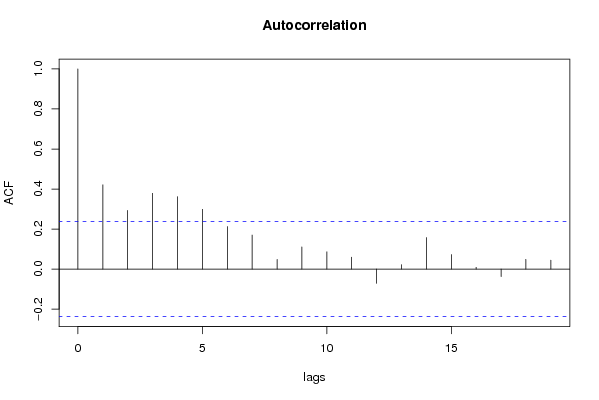
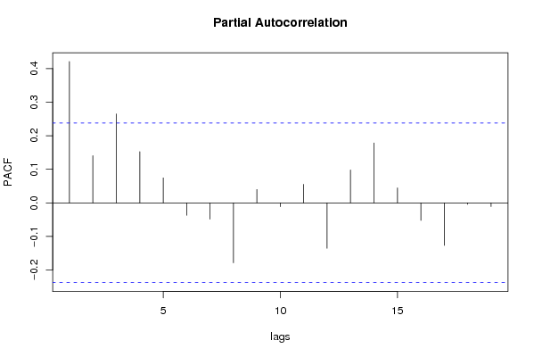
Title produced by software

(Partial) Autocorrelation Function

Date of computation

Fri, 23 Nov 2007 03:25:42 -0700

Cite this page as follows

Statistical Computations at FreeStatistics.org, Office for Research Development and Education, URL https://freestatistics.org/blog/index.php?v=date/2007/Nov/23/t119581303693qhxocpz6a2rbt.htm/, Retrieved Sun, 28 Apr 2024 20:09:26 +0000

Statistical Computations at FreeStatistics.org, Office for Research Development and Education, URL https://freestatistics.org/blog/index.php?pk=6133, Retrieved Sun, 28 Apr 2024 20:09:26 +0000

QR Codes:

Paste this QR Code to cite your computation.

Original text written by user:

IsPrivate?

No (this computation is public)

User-defined keywords

Q2, groep 1

Estimated Impact

218

Family? (F = Feedback message, R = changed R code, M = changed R Module, P = changed Parameters, D = changed Data)

-       [(Partial) Autocorrelation Function] [Q2, groep 1] [2007-11-23 10:25:42] [ce556af355e2eff84137e549c6ea8397] [Current]

Feedback Forum

Post a new message

Dataseries X:

Download CSV

Histogram

Boxplots

Summary of compuational transaction
Raw Input	view raw input (R code)
Raw Output	view raw output of R engine
Computing time	1 seconds
R Server	'Gwilym Jenkins' @ 72.249.127.135

\begin{tabular}{lllllllll}
\hline
Summary of compuational transaction \tabularnewline
Raw Input & view raw input (R code)  \tabularnewline
Raw Output & view raw output of R engine  \tabularnewline
Computing time & 1 seconds \tabularnewline
R Server & 'Gwilym Jenkins' @ 72.249.127.135 \tabularnewline
\hline
\end{tabular}
%Source: https://freestatistics.org/blog/index.php?pk=6133&T=0

[TABLE]
[ROW][C]Summary of compuational transaction[/C][/ROW]
[ROW][C]Raw Input[/C][C]view raw input (R code) [/C][/ROW]
[ROW][C]Raw Output[/C][C]view raw output of R engine [/C][/ROW]
[ROW][C]Computing time[/C][C]1 seconds[/C][/ROW]
[ROW][C]R Server[/C][C]'Gwilym Jenkins' @ 72.249.127.135[/C][/ROW]
[/TABLE]
Source: https://freestatistics.org/blog/index.php?pk=6133&T=0

Globally Unique Identifier (entire table): ba.freestatistics.org/blog/index.php?pk=6133&T=0

As an alternative you can also use a QR Code:

The GUIDs for individual cells are displayed in the table below:

Summary of compuational transaction
Raw Input	view raw input (R code)
Raw Output	view raw output of R engine
Computing time	1 seconds
R Server	'Gwilym Jenkins' @ 72.249.127.135

Autocorrelation Function
Time lag k	ACF(k)	T-STAT	P-value
0	1	8.2462	0
1	0.420905	3.4709	0.000453
2	0.29281	2.4146	0.009225
3	0.37872	3.123	0.001315
4	0.36186	2.984	0.001975
5	0.298768	2.4637	0.008143
6	0.212786	1.7547	0.04191
7	0.170285	1.4042	0.082405
8	0.048023	0.396	0.34667
9	0.110708	0.9129	0.182254
10	0.086313	0.7118	0.239526
11	0.059288	0.4889	0.313242
12	-0.070835	-0.5841	0.719465
13	0.022021	0.1816	0.428223
14	0.157333	1.2974	0.099438
15	0.072439	0.5974	0.276129
16	0.00903	0.0745	0.470429
17	-0.037195	-0.3067	0.620001
18	0.048534	0.4002	0.345125

\begin{tabular}{lllllllll}
\hline
Autocorrelation Function \tabularnewline
Time lag k & ACF(k) & T-STAT & P-value \tabularnewline
0 & 1 & 8.2462 & 0 \tabularnewline
1 & 0.420905 & 3.4709 & 0.000453 \tabularnewline
2 & 0.29281 & 2.4146 & 0.009225 \tabularnewline
3 & 0.37872 & 3.123 & 0.001315 \tabularnewline
4 & 0.36186 & 2.984 & 0.001975 \tabularnewline
5 & 0.298768 & 2.4637 & 0.008143 \tabularnewline
6 & 0.212786 & 1.7547 & 0.04191 \tabularnewline
7 & 0.170285 & 1.4042 & 0.082405 \tabularnewline
8 & 0.048023 & 0.396 & 0.34667 \tabularnewline
9 & 0.110708 & 0.9129 & 0.182254 \tabularnewline
10 & 0.086313 & 0.7118 & 0.239526 \tabularnewline
11 & 0.059288 & 0.4889 & 0.313242 \tabularnewline
12 & -0.070835 & -0.5841 & 0.719465 \tabularnewline
13 & 0.022021 & 0.1816 & 0.428223 \tabularnewline
14 & 0.157333 & 1.2974 & 0.099438 \tabularnewline
15 & 0.072439 & 0.5974 & 0.276129 \tabularnewline
16 & 0.00903 & 0.0745 & 0.470429 \tabularnewline
17 & -0.037195 & -0.3067 & 0.620001 \tabularnewline
18 & 0.048534 & 0.4002 & 0.345125 \tabularnewline
\hline
\end{tabular}
%Source: https://freestatistics.org/blog/index.php?pk=6133&T=1

[TABLE]
[ROW][C]Autocorrelation Function[/C][/ROW]
[ROW][C]Time lag k[/C][C]ACF(k)[/C][C]T-STAT[/C][C]P-value[/C][/ROW]
[ROW][C]0[/C][C]1[/C][C]8.2462[/C][C]0[/C][/ROW]
[ROW][C]1[/C][C]0.420905[/C][C]3.4709[/C][C]0.000453[/C][/ROW]
[ROW][C]2[/C][C]0.29281[/C][C]2.4146[/C][C]0.009225[/C][/ROW]
[ROW][C]3[/C][C]0.37872[/C][C]3.123[/C][C]0.001315[/C][/ROW]
[ROW][C]4[/C][C]0.36186[/C][C]2.984[/C][C]0.001975[/C][/ROW]
[ROW][C]5[/C][C]0.298768[/C][C]2.4637[/C][C]0.008143[/C][/ROW]
[ROW][C]6[/C][C]0.212786[/C][C]1.7547[/C][C]0.04191[/C][/ROW]
[ROW][C]7[/C][C]0.170285[/C][C]1.4042[/C][C]0.082405[/C][/ROW]
[ROW][C]8[/C][C]0.048023[/C][C]0.396[/C][C]0.34667[/C][/ROW]
[ROW][C]9[/C][C]0.110708[/C][C]0.9129[/C][C]0.182254[/C][/ROW]
[ROW][C]10[/C][C]0.086313[/C][C]0.7118[/C][C]0.239526[/C][/ROW]
[ROW][C]11[/C][C]0.059288[/C][C]0.4889[/C][C]0.313242[/C][/ROW]
[ROW][C]12[/C][C]-0.070835[/C][C]-0.5841[/C][C]0.719465[/C][/ROW]
[ROW][C]13[/C][C]0.022021[/C][C]0.1816[/C][C]0.428223[/C][/ROW]
[ROW][C]14[/C][C]0.157333[/C][C]1.2974[/C][C]0.099438[/C][/ROW]
[ROW][C]15[/C][C]0.072439[/C][C]0.5974[/C][C]0.276129[/C][/ROW]
[ROW][C]16[/C][C]0.00903[/C][C]0.0745[/C][C]0.470429[/C][/ROW]
[ROW][C]17[/C][C]-0.037195[/C][C]-0.3067[/C][C]0.620001[/C][/ROW]
[ROW][C]18[/C][C]0.048534[/C][C]0.4002[/C][C]0.345125[/C][/ROW]
[/TABLE]
Source: https://freestatistics.org/blog/index.php?pk=6133&T=1

Globally Unique Identifier (entire table): ba.freestatistics.org/blog/index.php?pk=6133&T=1

As an alternative you can also use a QR Code:

The GUIDs for individual cells are displayed in the table below:

Autocorrelation Function
Time lag k	ACF(k)	T-STAT	P-value
0	1	8.2462	0
1	0.420905	3.4709	0.000453
2	0.29281	2.4146	0.009225
3	0.37872	3.123	0.001315
4	0.36186	2.984	0.001975
5	0.298768	2.4637	0.008143
6	0.212786	1.7547	0.04191
7	0.170285	1.4042	0.082405
8	0.048023	0.396	0.34667
9	0.110708	0.9129	0.182254
10	0.086313	0.7118	0.239526
11	0.059288	0.4889	0.313242
12	-0.070835	-0.5841	0.719465
13	0.022021	0.1816	0.428223
14	0.157333	1.2974	0.099438
15	0.072439	0.5974	0.276129
16	0.00903	0.0745	0.470429
17	-0.037195	-0.3067	0.620001
18	0.048534	0.4002	0.345125

Partial Autocorrelation Function
Time lag k	PACF(k)	T-STAT	P-value
0	0.420905	3.4709	0.000453
1	0.140548	1.159	0.125257
2	0.264869	2.1842	0.016201
3	0.1525	1.2575	0.106429
4	0.074182	0.6117	0.271382
5	-0.036881	-0.3041	0.61902
6	-0.04856	-0.4004	0.654955
7	-0.178738	-1.4739	0.92744
8	0.039691	0.3273	0.372224
9	-0.011336	-0.0935	0.537102
10	0.055107	0.4544	0.325486
11	-0.135281	-1.1156	0.86573
12	0.097802	0.8065	0.211384
13	0.178444	1.4715	0.072886
14	0.044354	0.3658	0.357841
15	-0.052247	-0.4308	0.666028
16	-0.126881	-1.0463	0.850434
17	-0.004598	-0.0379	0.515068
18	-0.011037	-0.091	0.536127

\begin{tabular}{lllllllll}
\hline
Partial Autocorrelation Function \tabularnewline
Time lag k & PACF(k) & T-STAT & P-value \tabularnewline
0 & 0.420905 & 3.4709 & 0.000453 \tabularnewline
1 & 0.140548 & 1.159 & 0.125257 \tabularnewline
2 & 0.264869 & 2.1842 & 0.016201 \tabularnewline
3 & 0.1525 & 1.2575 & 0.106429 \tabularnewline
4 & 0.074182 & 0.6117 & 0.271382 \tabularnewline
5 & -0.036881 & -0.3041 & 0.61902 \tabularnewline
6 & -0.04856 & -0.4004 & 0.654955 \tabularnewline
7 & -0.178738 & -1.4739 & 0.92744 \tabularnewline
8 & 0.039691 & 0.3273 & 0.372224 \tabularnewline
9 & -0.011336 & -0.0935 & 0.537102 \tabularnewline
10 & 0.055107 & 0.4544 & 0.325486 \tabularnewline
11 & -0.135281 & -1.1156 & 0.86573 \tabularnewline
12 & 0.097802 & 0.8065 & 0.211384 \tabularnewline
13 & 0.178444 & 1.4715 & 0.072886 \tabularnewline
14 & 0.044354 & 0.3658 & 0.357841 \tabularnewline
15 & -0.052247 & -0.4308 & 0.666028 \tabularnewline
16 & -0.126881 & -1.0463 & 0.850434 \tabularnewline
17 & -0.004598 & -0.0379 & 0.515068 \tabularnewline
18 & -0.011037 & -0.091 & 0.536127 \tabularnewline
\hline
\end{tabular}
%Source: https://freestatistics.org/blog/index.php?pk=6133&T=2

[TABLE]
[ROW][C]Partial Autocorrelation Function[/C][/ROW]
[ROW][C]Time lag k[/C][C]PACF(k)[/C][C]T-STAT[/C][C]P-value[/C][/ROW]
[ROW][C]0[/C][C]0.420905[/C][C]3.4709[/C][C]0.000453[/C][/ROW]
[ROW][C]1[/C][C]0.140548[/C][C]1.159[/C][C]0.125257[/C][/ROW]
[ROW][C]2[/C][C]0.264869[/C][C]2.1842[/C][C]0.016201[/C][/ROW]
[ROW][C]3[/C][C]0.1525[/C][C]1.2575[/C][C]0.106429[/C][/ROW]
[ROW][C]4[/C][C]0.074182[/C][C]0.6117[/C][C]0.271382[/C][/ROW]
[ROW][C]5[/C][C]-0.036881[/C][C]-0.3041[/C][C]0.61902[/C][/ROW]
[ROW][C]6[/C][C]-0.04856[/C][C]-0.4004[/C][C]0.654955[/C][/ROW]
[ROW][C]7[/C][C]-0.178738[/C][C]-1.4739[/C][C]0.92744[/C][/ROW]
[ROW][C]8[/C][C]0.039691[/C][C]0.3273[/C][C]0.372224[/C][/ROW]
[ROW][C]9[/C][C]-0.011336[/C][C]-0.0935[/C][C]0.537102[/C][/ROW]
[ROW][C]10[/C][C]0.055107[/C][C]0.4544[/C][C]0.325486[/C][/ROW]
[ROW][C]11[/C][C]-0.135281[/C][C]-1.1156[/C][C]0.86573[/C][/ROW]
[ROW][C]12[/C][C]0.097802[/C][C]0.8065[/C][C]0.211384[/C][/ROW]
[ROW][C]13[/C][C]0.178444[/C][C]1.4715[/C][C]0.072886[/C][/ROW]
[ROW][C]14[/C][C]0.044354[/C][C]0.3658[/C][C]0.357841[/C][/ROW]
[ROW][C]15[/C][C]-0.052247[/C][C]-0.4308[/C][C]0.666028[/C][/ROW]
[ROW][C]16[/C][C]-0.126881[/C][C]-1.0463[/C][C]0.850434[/C][/ROW]
[ROW][C]17[/C][C]-0.004598[/C][C]-0.0379[/C][C]0.515068[/C][/ROW]
[ROW][C]18[/C][C]-0.011037[/C][C]-0.091[/C][C]0.536127[/C][/ROW]
[/TABLE]
Source: https://freestatistics.org/blog/index.php?pk=6133&T=2

Globally Unique Identifier (entire table): ba.freestatistics.org/blog/index.php?pk=6133&T=2

As an alternative you can also use a QR Code:

The GUIDs for individual cells are displayed in the table below:

Partial Autocorrelation Function
Time lag k	PACF(k)	T-STAT	P-value
0	0.420905	3.4709	0.000453
1	0.140548	1.159	0.125257
2	0.264869	2.1842	0.016201
3	0.1525	1.2575	0.106429
4	0.074182	0.6117	0.271382
5	-0.036881	-0.3041	0.61902
6	-0.04856	-0.4004	0.654955
7	-0.178738	-1.4739	0.92744
8	0.039691	0.3273	0.372224
9	-0.011336	-0.0935	0.537102
10	0.055107	0.4544	0.325486
11	-0.135281	-1.1156	0.86573
12	0.097802	0.8065	0.211384
13	0.178444	1.4715	0.072886
14	0.044354	0.3658	0.357841
15	-0.052247	-0.4308	0.666028
16	-0.126881	-1.0463	0.850434
17	-0.004598	-0.0379	0.515068
18	-0.011037	-0.091	0.536127

Figure 1

PNG link

Postscript link

PDF link

Figure 2

PNG link

Postscript link

PDF link

Parameters (Session):

par1 = Default ; par2 = 1 ; par3 = 0 ; par4 = 1 ; par5 = 12 ;

Parameters (R input):

par1 = Default ; par2 = 1 ; par3 = 0 ; par4 = 1 ; par5 = 12 ;

R code (references can be found in the software module):

if (par1 == 'Default') {
par1 = 10*log10(length(x))
} else {
par1 <- as.numeric(par1)
}
par2 <- as.numeric(par2)
par3 <- as.numeric(par3)
par4 <- as.numeric(par4)
par5 <- as.numeric(par5)
if (par2 == 0) {
x <- log(x)
} else {
x <- (x ^ par2 - 1) / par2
}
if (par3 > 0) x <- diff(x,lag=1,difference=par3)
if (par4 > 0) x <- diff(x,lag=par5,difference=par4)
bitmap(file='pic1.png')
racf <- acf(x,par1,main='Autocorrelation',xlab='lags',ylab='ACF')
dev.off()
bitmap(file='pic2.png')
rpacf <- pacf(x,par1,main='Partial Autocorrelation',xlab='lags',ylab='PACF')
dev.off()
(myacf <- c(racf$acf))
(mypacf <- c(rpacf$acf))
lengthx <- length(x)
sqrtn <- sqrt(lengthx)
load(file='createtable')
a<-table.start()
a<-table.row.start(a)
a<-table.element(a,'Autocorrelation Function',4,TRUE)
a<-table.row.end(a)
a<-table.row.start(a)
a<-table.element(a,'Time lag k',header=TRUE)
a<-table.element(a,hyperlink('basics.htm','ACF(k)','click here for more information about the Autocorrelation Function'),header=TRUE)
a<-table.element(a,'T-STAT',header=TRUE)
a<-table.element(a,'P-value',header=TRUE)
a<-table.row.end(a)
for (i in 1:par1) {
a<-table.row.start(a)
a<-table.element(a,i-1,header=TRUE)
a<-table.element(a,round(myacf[i],6))
mytstat <- myacf[i]*sqrtn
a<-table.element(a,round(mytstat,4))
a<-table.element(a,round(1-pt(mytstat,lengthx),6))
a<-table.row.end(a)
}
a<-table.end(a)
table.save(a,file='mytable.tab')
a<-table.start()
a<-table.row.start(a)
a<-table.element(a,'Partial Autocorrelation Function',4,TRUE)
a<-table.row.end(a)
a<-table.row.start(a)
a<-table.element(a,'Time lag k',header=TRUE)
a<-table.element(a,hyperlink('basics.htm','PACF(k)','click here for more information about the Partial Autocorrelation Function'),header=TRUE)
a<-table.element(a,'T-STAT',header=TRUE)
a<-table.element(a,'P-value',header=TRUE)
a<-table.row.end(a)
for (i in 1:par1) {
a<-table.row.start(a)
a<-table.element(a,i-1,header=TRUE)
a<-table.element(a,round(mypacf[i],6))
mytstat <- mypacf[i]*sqrtn
a<-table.element(a,round(mytstat,4))
a<-table.element(a,round(1-pt(mytstat,lengthx),6))
a<-table.row.end(a)
}
a<-table.end(a)
table.save(a,file='mytable1.tab')

Free Statistics

Description of Statistical Computation

Tree of Dependent Computations

Dataset

Tables (Output of Computation)

Figures (Output of Computation)

Input Parameters & R Code