Repository of Reproducible Computations

Free Statistics

of Irreproducible Research!

Author's title

Author

*Unverified author*

R Software Module

rwasp_autocorrelation.wasp

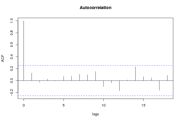
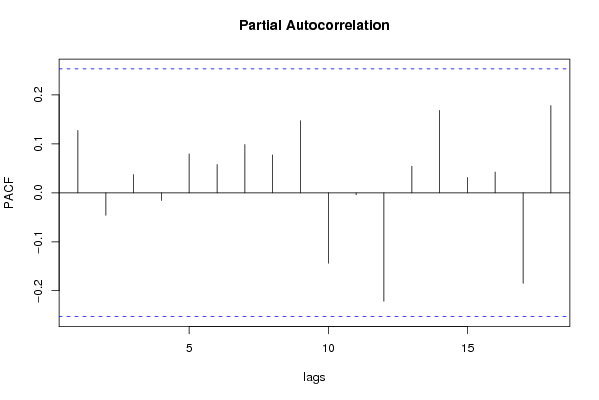
Title produced by software

(Partial) Autocorrelation Function

Date of computation

Thu, 22 Nov 2007 06:00:02 -0700

Cite this page as follows

Statistical Computations at FreeStatistics.org, Office for Research Development and Education, URL https://freestatistics.org/blog/index.php?v=date/2007/Nov/22/t1195735944oz7rbo9jug2oe1e.htm/, Retrieved Thu, 02 May 2024 14:45:51 +0000

Statistical Computations at FreeStatistics.org, Office for Research Development and Education, URL https://freestatistics.org/blog/index.php?pk=5961, Retrieved Thu, 02 May 2024 14:45:51 +0000

QR Codes:

Paste this QR Code to cite your computation.

Original text written by user:

IsPrivate?

No (this computation is public)

User-defined keywords

Estimated Impact

232

Family? (F = Feedback message, R = changed R code, M = changed R Module, P = changed Parameters, D = changed Data)

-       [(Partial) Autocorrelation Function] [Partiel Autocorre...] [2007-11-22 13:00:02] [2cdb7403ed3391afb545b8c0d20da37e] [Current]
-   PD    [(Partial) Autocorrelation Function] [WS 9] [2007-11-23 13:25:45] [74be16979710d4c4e7c6647856088456] 
-   PD    [(Partial) Autocorrelation Function] [WS 9] [2007-11-23 13:33:33] [74be16979710d4c4e7c6647856088456] 
-   PD    [(Partial) Autocorrelation Function] [WS 9] [2007-11-23 13:37:14] [74be16979710d4c4e7c6647856088456] 
-   PD    [(Partial) Autocorrelation Function] [WS 9] [2007-11-23 13:37:14] [74be16979710d4c4e7c6647856088456] 
-    D    [(Partial) Autocorrelation Function] [WS 9] [2007-11-23 13:41:40] [74be16979710d4c4e7c6647856088456] 
- RMPD    [Spectral Analysis] [WS 9 Spectral ana...] [2007-11-23 13:44:44] [74be16979710d4c4e7c6647856088456] 
- RMPD    [Spectral Analysis] [WS 9] [2007-11-23 13:55:37] [74be16979710d4c4e7c6647856088456] 
- RMPD    [Spectral Analysis] [ws9] [2007-11-23 13:59:41] [74be16979710d4c4e7c6647856088456] 
- RMPD    [Spectral Analysis] [WS 9] [2007-11-23 14:04:33] [74be16979710d4c4e7c6647856088456] 
- RMPD    [Spectral Analysis] [WS 9] [2007-11-23 14:04:33] [74be16979710d4c4e7c6647856088456] 
- RMPD    [Spectral Analysis] [ws9] [2007-11-23 14:07:55] [74be16979710d4c4e7c6647856088456] 
- RMPD    [Spectral Analysis] [ws 9] [2007-11-23 14:10:12] [74be16979710d4c4e7c6647856088456] 
- RMPD    [Spectral Analysis] [ws 9] [2007-11-23 14:14:56] [74be16979710d4c4e7c6647856088456] 
- RMPD    [Variance Reduction Matrix] [ws9] [2007-11-23 14:18:32] [74be16979710d4c4e7c6647856088456] 

Feedback Forum

Post a new message

Dataseries X:

Download CSV

Histogram

Boxplots

Summary of compuational transaction
Raw Input	view raw input (R code)
Raw Output	view raw output of R engine
Computing time	2 seconds
R Server	'Gwilym Jenkins' @ 72.249.127.135

\begin{tabular}{lllllllll}
\hline
Summary of compuational transaction \tabularnewline
Raw Input & view raw input (R code)  \tabularnewline
Raw Output & view raw output of R engine  \tabularnewline
Computing time & 2 seconds \tabularnewline
R Server & 'Gwilym Jenkins' @ 72.249.127.135 \tabularnewline
\hline
\end{tabular}
%Source: https://freestatistics.org/blog/index.php?pk=5961&T=0

[TABLE]
[ROW][C]Summary of compuational transaction[/C][/ROW]
[ROW][C]Raw Input[/C][C]view raw input (R code) [/C][/ROW]
[ROW][C]Raw Output[/C][C]view raw output of R engine [/C][/ROW]
[ROW][C]Computing time[/C][C]2 seconds[/C][/ROW]
[ROW][C]R Server[/C][C]'Gwilym Jenkins' @ 72.249.127.135[/C][/ROW]
[/TABLE]
Source: https://freestatistics.org/blog/index.php?pk=5961&T=0

Globally Unique Identifier (entire table): ba.freestatistics.org/blog/index.php?pk=5961&T=0

As an alternative you can also use a QR Code:

The GUIDs for individual cells are displayed in the table below:

Summary of compuational transaction
Raw Input	view raw input (R code)
Raw Output	view raw output of R engine
Computing time	2 seconds
R Server	'Gwilym Jenkins' @ 72.249.127.135

Autocorrelation Function
Time lag k	ACF(k)	T-STAT	P-value
0	1	7.746	0
1	0.127423	0.987	0.163801
2	-0.028998	-0.2246	0.58848
3	0.026844	0.2079	0.417992
4	-0.005511	-0.0427	0.516954
5	0.072436	0.5611	0.288414
6	0.078338	0.6068	0.273136
7	0.106676	0.8263	0.205951
8	0.099701	0.7723	0.221491
9	0.155056	1.2011	0.117224
10	-0.100006	-0.7746	0.779203
11	-0.038676	-0.2996	0.617235
12	-0.169341	-1.3117	0.902693
13	0.013332	0.1033	0.459046
14	0.228576	1.7705	0.040858
15	0.067221	0.5207	0.302248
16	0.048894	0.3787	0.353111
17	-0.162511	-1.2588	0.893512

\begin{tabular}{lllllllll}
\hline
Autocorrelation Function \tabularnewline
Time lag k & ACF(k) & T-STAT & P-value \tabularnewline
0 & 1 & 7.746 & 0 \tabularnewline
1 & 0.127423 & 0.987 & 0.163801 \tabularnewline
2 & -0.028998 & -0.2246 & 0.58848 \tabularnewline
3 & 0.026844 & 0.2079 & 0.417992 \tabularnewline
4 & -0.005511 & -0.0427 & 0.516954 \tabularnewline
5 & 0.072436 & 0.5611 & 0.288414 \tabularnewline
6 & 0.078338 & 0.6068 & 0.273136 \tabularnewline
7 & 0.106676 & 0.8263 & 0.205951 \tabularnewline
8 & 0.099701 & 0.7723 & 0.221491 \tabularnewline
9 & 0.155056 & 1.2011 & 0.117224 \tabularnewline
10 & -0.100006 & -0.7746 & 0.779203 \tabularnewline
11 & -0.038676 & -0.2996 & 0.617235 \tabularnewline
12 & -0.169341 & -1.3117 & 0.902693 \tabularnewline
13 & 0.013332 & 0.1033 & 0.459046 \tabularnewline
14 & 0.228576 & 1.7705 & 0.040858 \tabularnewline
15 & 0.067221 & 0.5207 & 0.302248 \tabularnewline
16 & 0.048894 & 0.3787 & 0.353111 \tabularnewline
17 & -0.162511 & -1.2588 & 0.893512 \tabularnewline
\hline
\end{tabular}
%Source: https://freestatistics.org/blog/index.php?pk=5961&T=1

[TABLE]
[ROW][C]Autocorrelation Function[/C][/ROW]
[ROW][C]Time lag k[/C][C]ACF(k)[/C][C]T-STAT[/C][C]P-value[/C][/ROW]
[ROW][C]0[/C][C]1[/C][C]7.746[/C][C]0[/C][/ROW]
[ROW][C]1[/C][C]0.127423[/C][C]0.987[/C][C]0.163801[/C][/ROW]
[ROW][C]2[/C][C]-0.028998[/C][C]-0.2246[/C][C]0.58848[/C][/ROW]
[ROW][C]3[/C][C]0.026844[/C][C]0.2079[/C][C]0.417992[/C][/ROW]
[ROW][C]4[/C][C]-0.005511[/C][C]-0.0427[/C][C]0.516954[/C][/ROW]
[ROW][C]5[/C][C]0.072436[/C][C]0.5611[/C][C]0.288414[/C][/ROW]
[ROW][C]6[/C][C]0.078338[/C][C]0.6068[/C][C]0.273136[/C][/ROW]
[ROW][C]7[/C][C]0.106676[/C][C]0.8263[/C][C]0.205951[/C][/ROW]
[ROW][C]8[/C][C]0.099701[/C][C]0.7723[/C][C]0.221491[/C][/ROW]
[ROW][C]9[/C][C]0.155056[/C][C]1.2011[/C][C]0.117224[/C][/ROW]
[ROW][C]10[/C][C]-0.100006[/C][C]-0.7746[/C][C]0.779203[/C][/ROW]
[ROW][C]11[/C][C]-0.038676[/C][C]-0.2996[/C][C]0.617235[/C][/ROW]
[ROW][C]12[/C][C]-0.169341[/C][C]-1.3117[/C][C]0.902693[/C][/ROW]
[ROW][C]13[/C][C]0.013332[/C][C]0.1033[/C][C]0.459046[/C][/ROW]
[ROW][C]14[/C][C]0.228576[/C][C]1.7705[/C][C]0.040858[/C][/ROW]
[ROW][C]15[/C][C]0.067221[/C][C]0.5207[/C][C]0.302248[/C][/ROW]
[ROW][C]16[/C][C]0.048894[/C][C]0.3787[/C][C]0.353111[/C][/ROW]
[ROW][C]17[/C][C]-0.162511[/C][C]-1.2588[/C][C]0.893512[/C][/ROW]
[/TABLE]
Source: https://freestatistics.org/blog/index.php?pk=5961&T=1

Globally Unique Identifier (entire table): ba.freestatistics.org/blog/index.php?pk=5961&T=1

As an alternative you can also use a QR Code:

The GUIDs for individual cells are displayed in the table below:

Autocorrelation Function
Time lag k	ACF(k)	T-STAT	P-value
0	1	7.746	0
1	0.127423	0.987	0.163801
2	-0.028998	-0.2246	0.58848
3	0.026844	0.2079	0.417992
4	-0.005511	-0.0427	0.516954
5	0.072436	0.5611	0.288414
6	0.078338	0.6068	0.273136
7	0.106676	0.8263	0.205951
8	0.099701	0.7723	0.221491
9	0.155056	1.2011	0.117224
10	-0.100006	-0.7746	0.779203
11	-0.038676	-0.2996	0.617235
12	-0.169341	-1.3117	0.902693
13	0.013332	0.1033	0.459046
14	0.228576	1.7705	0.040858
15	0.067221	0.5207	0.302248
16	0.048894	0.3787	0.353111
17	-0.162511	-1.2588	0.893512

Partial Autocorrelation Function
Time lag k	PACF(k)	T-STAT	P-value
0	0.127423	0.987	0.163801
1	-0.045981	-0.3562	0.638518
2	0.03725	0.2885	0.386964
3	-0.015667	-0.1214	0.548093
4	0.079289	0.6142	0.270712
5	0.057591	0.4461	0.328567
6	0.098654	0.7642	0.22388
7	0.077304	0.5988	0.275782
8	0.14727	1.1407	0.129254
9	-0.143793	-1.1138	0.865101
10	-0.004198	-0.0325	0.512916
11	-0.221445	-1.7153	0.954275
12	0.05431	0.4207	0.337746
13	0.168242	1.3032	0.098743
14	0.031468	0.2437	0.404129
15	0.042419	0.3286	0.371811
16	-0.18484	-1.4318	0.9213
17	0.178263	1.3808	0.086228

\begin{tabular}{lllllllll}
\hline
Partial Autocorrelation Function \tabularnewline
Time lag k & PACF(k) & T-STAT & P-value \tabularnewline
0 & 0.127423 & 0.987 & 0.163801 \tabularnewline
1 & -0.045981 & -0.3562 & 0.638518 \tabularnewline
2 & 0.03725 & 0.2885 & 0.386964 \tabularnewline
3 & -0.015667 & -0.1214 & 0.548093 \tabularnewline
4 & 0.079289 & 0.6142 & 0.270712 \tabularnewline
5 & 0.057591 & 0.4461 & 0.328567 \tabularnewline
6 & 0.098654 & 0.7642 & 0.22388 \tabularnewline
7 & 0.077304 & 0.5988 & 0.275782 \tabularnewline
8 & 0.14727 & 1.1407 & 0.129254 \tabularnewline
9 & -0.143793 & -1.1138 & 0.865101 \tabularnewline
10 & -0.004198 & -0.0325 & 0.512916 \tabularnewline
11 & -0.221445 & -1.7153 & 0.954275 \tabularnewline
12 & 0.05431 & 0.4207 & 0.337746 \tabularnewline
13 & 0.168242 & 1.3032 & 0.098743 \tabularnewline
14 & 0.031468 & 0.2437 & 0.404129 \tabularnewline
15 & 0.042419 & 0.3286 & 0.371811 \tabularnewline
16 & -0.18484 & -1.4318 & 0.9213 \tabularnewline
17 & 0.178263 & 1.3808 & 0.086228 \tabularnewline
\hline
\end{tabular}
%Source: https://freestatistics.org/blog/index.php?pk=5961&T=2

[TABLE]
[ROW][C]Partial Autocorrelation Function[/C][/ROW]
[ROW][C]Time lag k[/C][C]PACF(k)[/C][C]T-STAT[/C][C]P-value[/C][/ROW]
[ROW][C]0[/C][C]0.127423[/C][C]0.987[/C][C]0.163801[/C][/ROW]
[ROW][C]1[/C][C]-0.045981[/C][C]-0.3562[/C][C]0.638518[/C][/ROW]
[ROW][C]2[/C][C]0.03725[/C][C]0.2885[/C][C]0.386964[/C][/ROW]
[ROW][C]3[/C][C]-0.015667[/C][C]-0.1214[/C][C]0.548093[/C][/ROW]
[ROW][C]4[/C][C]0.079289[/C][C]0.6142[/C][C]0.270712[/C][/ROW]
[ROW][C]5[/C][C]0.057591[/C][C]0.4461[/C][C]0.328567[/C][/ROW]
[ROW][C]6[/C][C]0.098654[/C][C]0.7642[/C][C]0.22388[/C][/ROW]
[ROW][C]7[/C][C]0.077304[/C][C]0.5988[/C][C]0.275782[/C][/ROW]
[ROW][C]8[/C][C]0.14727[/C][C]1.1407[/C][C]0.129254[/C][/ROW]
[ROW][C]9[/C][C]-0.143793[/C][C]-1.1138[/C][C]0.865101[/C][/ROW]
[ROW][C]10[/C][C]-0.004198[/C][C]-0.0325[/C][C]0.512916[/C][/ROW]
[ROW][C]11[/C][C]-0.221445[/C][C]-1.7153[/C][C]0.954275[/C][/ROW]
[ROW][C]12[/C][C]0.05431[/C][C]0.4207[/C][C]0.337746[/C][/ROW]
[ROW][C]13[/C][C]0.168242[/C][C]1.3032[/C][C]0.098743[/C][/ROW]
[ROW][C]14[/C][C]0.031468[/C][C]0.2437[/C][C]0.404129[/C][/ROW]
[ROW][C]15[/C][C]0.042419[/C][C]0.3286[/C][C]0.371811[/C][/ROW]
[ROW][C]16[/C][C]-0.18484[/C][C]-1.4318[/C][C]0.9213[/C][/ROW]
[ROW][C]17[/C][C]0.178263[/C][C]1.3808[/C][C]0.086228[/C][/ROW]
[/TABLE]
Source: https://freestatistics.org/blog/index.php?pk=5961&T=2

Globally Unique Identifier (entire table): ba.freestatistics.org/blog/index.php?pk=5961&T=2

As an alternative you can also use a QR Code:

The GUIDs for individual cells are displayed in the table below:

Partial Autocorrelation Function
Time lag k	PACF(k)	T-STAT	P-value
0	0.127423	0.987	0.163801
1	-0.045981	-0.3562	0.638518
2	0.03725	0.2885	0.386964
3	-0.015667	-0.1214	0.548093
4	0.079289	0.6142	0.270712
5	0.057591	0.4461	0.328567
6	0.098654	0.7642	0.22388
7	0.077304	0.5988	0.275782
8	0.14727	1.1407	0.129254
9	-0.143793	-1.1138	0.865101
10	-0.004198	-0.0325	0.512916
11	-0.221445	-1.7153	0.954275
12	0.05431	0.4207	0.337746
13	0.168242	1.3032	0.098743
14	0.031468	0.2437	0.404129
15	0.042419	0.3286	0.371811
16	-0.18484	-1.4318	0.9213
17	0.178263	1.3808	0.086228

Figure 1

PNG link

Postscript link

PDF link

Figure 2

PNG link

Postscript link

PDF link

Parameters (Session):

par1 = Default ; par2 = 1 ; par3 = 1 ; par4 = 1 ; par5 = 12 ;

Parameters (R input):

par1 = Default ; par2 = 1 ; par3 = 1 ; par4 = 1 ; par5 = 12 ;

R code (references can be found in the software module):

if (par1 == 'Default') {
par1 = 10*log10(length(x))
} else {
par1 <- as.numeric(par1)
}
par2 <- as.numeric(par2)
par3 <- as.numeric(par3)
par4 <- as.numeric(par4)
par5 <- as.numeric(par5)
if (par2 == 0) {
x <- log(x)
} else {
x <- (x ^ par2 - 1) / par2
}
if (par3 > 0) x <- diff(x,lag=1,difference=par3)
if (par4 > 0) x <- diff(x,lag=par5,difference=par4)
bitmap(file='pic1.png')
racf <- acf(x,par1,main='Autocorrelation',xlab='lags',ylab='ACF')
dev.off()
bitmap(file='pic2.png')
rpacf <- pacf(x,par1,main='Partial Autocorrelation',xlab='lags',ylab='PACF')
dev.off()
(myacf <- c(racf$acf))
(mypacf <- c(rpacf$acf))
lengthx <- length(x)
sqrtn <- sqrt(lengthx)
load(file='createtable')
a<-table.start()
a<-table.row.start(a)
a<-table.element(a,'Autocorrelation Function',4,TRUE)
a<-table.row.end(a)
a<-table.row.start(a)
a<-table.element(a,'Time lag k',header=TRUE)
a<-table.element(a,hyperlink('basics.htm','ACF(k)','click here for more information about the Autocorrelation Function'),header=TRUE)
a<-table.element(a,'T-STAT',header=TRUE)
a<-table.element(a,'P-value',header=TRUE)
a<-table.row.end(a)
for (i in 1:par1) {
a<-table.row.start(a)
a<-table.element(a,i-1,header=TRUE)
a<-table.element(a,round(myacf[i],6))
mytstat <- myacf[i]*sqrtn
a<-table.element(a,round(mytstat,4))
a<-table.element(a,round(1-pt(mytstat,lengthx),6))
a<-table.row.end(a)
}
a<-table.end(a)
table.save(a,file='mytable.tab')
a<-table.start()
a<-table.row.start(a)
a<-table.element(a,'Partial Autocorrelation Function',4,TRUE)
a<-table.row.end(a)
a<-table.row.start(a)
a<-table.element(a,'Time lag k',header=TRUE)
a<-table.element(a,hyperlink('basics.htm','PACF(k)','click here for more information about the Partial Autocorrelation Function'),header=TRUE)
a<-table.element(a,'T-STAT',header=TRUE)
a<-table.element(a,'P-value',header=TRUE)
a<-table.row.end(a)
for (i in 1:par1) {
a<-table.row.start(a)
a<-table.element(a,i-1,header=TRUE)
a<-table.element(a,round(mypacf[i],6))
mytstat <- mypacf[i]*sqrtn
a<-table.element(a,round(mytstat,4))
a<-table.element(a,round(1-pt(mytstat,lengthx),6))
a<-table.row.end(a)
}
a<-table.end(a)
table.save(a,file='mytable1.tab')

Free Statistics

Description of Statistical Computation

Tree of Dependent Computations

Dataset

Tables (Output of Computation)

Figures (Output of Computation)

Input Parameters & R Code